|
|
| Line 1: |
Line 1: |
| − | Groundwater migrates from areas of higher [[wikipedia: Hydraulic head | hydraulic head]] toward lower hydraulic head, transporting dissolved solutes through the combined processes of [[wikipedia: Advection | advection]] and [[wikipedia: Dispersion | dispersion]]. Advection refers to the bulk movement of solutes carried by flowing groundwater. Dispersion refers to the spreading of the contaminant plume from highly concentrated areas to less concentrated areas. In many groundwater transport models, solute transport is described by the advection-dispersion-reaction equation in which dispersion coefficients can be calculated as the sum of molecular diffusion, mechanical dispersion, and macrodispersion.
| + | ==Estimating PCE/TCE Abiotic First-Order Reductive Dechlorination Rate Constants in Clayey Soils Under Anoxic Conditions== |
| − | | + | The U.S. Department of Defense (DoD) faces many challenges in restoring aquifers at contaminated sites, often due to back-diffusion of tetrachloroethene (PCE) and trichloroethene (TCE) from low-permeability clay zones. The uptake, storage, and subsequent long-term release of these dissolved contaminants from clays are key processes in understanding the longevity, intensity, and risks associated with many persistent chlorinated ethene groundwater plumes. Although naturally occurring abiotic and biotic dechlorination processes in clays may reduce stored contaminant mass and significantly aid natural attenuation, no standardized field method currently exists to verify or quantify these reactions. It is critical to remediation design efforts to demonstrate and validate a cost-effective in situ approach for assessing these dechlorination processes using first-order rate constants. An approach was developed and applied across eight DoD sites to support Remedial Project Managers (RPMs) and regulators in evaluating natural attenuation potential in clay-rich environments. |
| | <div style="float:right;margin:0 0 2em 2em;">__TOC__</div> | | <div style="float:right;margin:0 0 2em 2em;">__TOC__</div> |
| | | | |
| | '''Related Article(s):''' | | '''Related Article(s):''' |
| | | | |
| − | *[[Dispersion and Diffusion]] | + | *[[Monitored Natural Attenuation (MNA)]] |
| − | *[[Sorption of Organic Contaminants]] | + | *[[Monitored Natural Attenuation (MNA) of Chlorinated Solvents]] |
| − | *[[Plume Response Modeling]]
| + | *[[Monitored Natural Attenuation - Transitioning from Active Remedies]] |
| − | | + | *[[Matrix Diffusion]] |
| − | '''CONTRIBUTOR(S):''' [[Dr. Charles Newell, P.E.|Dr. Charles Newell]] and [[Dr. Robert Borden, P.E.|Dr. Robert Borden]]
| + | *[[REMChlor - MD]] |
| − | | |
| − | '''Key Resource(s):'''
| |
| − | | |
| − | *[http://hydrogeologistswithoutborders.org/wordpress/1979-english/ Groundwater]<ref name="FandC1979">Freeze, A., and Cherry, J., 1979. Groundwater, Prentice-Hall, Englewood Cliffs, New Jersey, 604 pages. Free download from [http://hydrogeologistswithoutborders.org/wordpress/1979-english/ Hydrogeologists Without Borders].</ref>, Freeze and Cherry, 1979. | |
| − | *[https://gw-project.org/books/hydrogeologic-properties-of-earth-materials-and-principles-of-groundwater-flow/ Hydrogeologic Properties of Earth Materials and Principals of Groundwater Flow]<ref name="Woessner2020">Woessner, W.W., and Poeter, E.P., 2020. Properties of Earth Materials and Principals of Groundwater Flow, The Groundwater Project, Guelph, Ontario, 207 pages. Free download from [https://gw-project.org/books/hydrogeologic-properties-of-earth-materials-and-principles-of-groundwater-flow/ The Groundwater Project].</ref>, Woessner and Poeter, 2020.
| |
| − | | |
| − | ==Groundwater Flow==
| |
| − | [[File:Newell-Article 1-Fig1r.JPG|thumbnail|left|400px|Figure 1. Hydraulic gradient (typically described in units of m/m or ft/ft) is the difference in hydraulic head from Point A to Point B (ΔH) divided by the distance between them (ΔL). In unconfined aquifers, the hydraulic gradient can also be described as the slope of the water table (Adapted from course notes developed by Dr. R.J. Mitchell, Western Washington University).]] | |
| − | Groundwater flows from areas of higher [[wikipedia: Hydraulic head | hydraulic head]] (a measure of pressure and gravitational energy) toward areas of lower hydraulic head (Figure 1). The rate of change (slope) of the hydraulic head is known as the hydraulic gradient. If groundwater is flowing and contains dissolved contaminants it can transport the contaminants by advection from areas with high hydraulic head toward lower hydraulic head zones, or “downgradient”.
| |
| − | | |
| − | ==Darcy's Law==
| |
| − | {| class="wikitable" style="float:right; margin-left:10px;text-align:center;"
| |
| − | |+Table 1. Representative values of total porosity (''n''), effective porosity (''n<sub>e</sub>''), and hydraulic conductivity (''K'') for different aquifer materials<ref name="D&S1997">Domenico, P.A. and Schwartz, F.W., 1997. Physical and Chemical Hydrogeology, 2nd Ed. John Wiley & Sons, 528 pgs. ISBN 978-0-471-59762-9. Available from: [https://www.wiley.com/en-us/Physical+and+Chemical+Hydrogeology%2C+2nd+Edition-p-9780471597629 Wiley]</ref><ref>McWhorter, D.B. and Sunada, D.K., 1977. Ground-water hydrology and hydraulics. Water Resources Publications, LLC, Highlands Ranch, Colorado, 304 pgs. ISBN-13: 978-1-887201-61-2 Available from: [https://www.wrpllc.com/books/gwhh.html Water Resources Publications]</ref><ref name="FandC1979" />
| |
| − | |-
| |
| − | !Aquifer Material
| |
| − | !Total Porosity<br /><small>(dimensionless)</small>
| |
| − | !Effective Porosity<br /><small>(dimensionless)</small>
| |
| − | !Hydraulic Conductivity<br /><small>(meters/second)</small>
| |
| − | |-
| |
| − | | colspan="4" style="text-align: left; background-color:white;" |'''Unconsolidated'''
| |
| − | |-
| |
| − | |Gravel||0.25 — 0.44||0.13 — 0.44||3×10<sup>-4</sup> — 3×10<sup>-2</sup>
| |
| − | |-
| |
| − | |Coarse Sand||0.31 — 0.46||0.18 — 0.43||9×10<sup>-7</sup> — 6×10<sup>-3</sup>
| |
| − | |-
| |
| − | |Medium Sand||—||0.16 — 0.46||9×10<sup>-7</sup> — 5×10<sup>-4</sup>
| |
| − | |-
| |
| − | |Fine Sand||0.25 — 0.53||0.01 — 0.46||2×10<sup>-7</sup> — 2×10<sup>-4</sup>
| |
| − | |-
| |
| − | |Silt, Loess||0.35 — 0.50||0.01 — 0.39||1×10<sup>-9</sup> — 2×10<sup>-5</sup>
| |
| − | |-
| |
| − | |Clay||0.40 — 0.70||0.01 — 0.18||1×10<sup>-11</sup> — 4.7×10<sup>-9</sup>
| |
| − | |-
| |
| − | | colspan="4" style="text-align: left; background-color:white;" |'''Sedimentary and Crystalline Rocks'''
| |
| − | |-
| |
| − | |Karst and Reef Limestone||0.05 — 0.50||—||1×10<sup>-6</sup> — 2×10<sup>-2</sup>
| |
| − | |-
| |
| − | |Limestone, Dolomite||0.00 — 0.20||0.01 — 0.24||1×10<sup>-9</sup> — 6×10<sup>-6</sup>
| |
| − | |-
| |
| − | |Sandstone||0.05 — 0.30||0.10 — 0.30||3×10<sup>-10</sup> — 6×10<sup>-6</sup>
| |
| − | |-
| |
| − | |Siltstone||—||0.21 — 0.41||1×10<sup>-11</sup> — 1.4×10<sup>-8</sup>
| |
| − | |-
| |
| − | |Basalt||0.05 — 0.50||—||2×10<sup>-11</sup> — 2×10<sup>-2</sup>
| |
| − | |-
| |
| − | |Fractured Crystalline Rock||0.00 — 0.10||—||8×10<sup>-9</sup> — 3×10<sup>-4</sup>
| |
| − | |-
| |
| − | |Weathered Granite||0.34 — 0.57||—||3.3×10<sup>-6</sup> — 5.2×10<sup>-5</sup>
| |
| − | |-
| |
| − | |Unfractured Crystalline Rock||0.00 — 0.05||—||3×10<sup>-14</sup> — 2×10<sup>-10</sup>
| |
| − | |}
| |
| − | In unconsolidated geologic settings (gravel, sand, silt, and clay) and highly fractured systems, the rate of groundwater movement can be expressed using [[wikipedia: Darcy's law | Darcy’s Law]]. This law is a fundamental mathematical relationship in the groundwater field and can be expressed this way:
| |
| | | | |
| − | [[File:Newell-Article 1-Equation 1rr.jpg|center|500px]]
| + | '''Contributors:''' Dani Tran, Dr. Charles Schaefer, Dr. Charles Werth |
| | | | |
| − | ::Where:
| + | '''Key Resource:''' |
| − | :::''Q'' = Flow rate (Volume of groundwater flow per time, such as m<sup>3</sup>/yr)
| + | *Schaefer, C.E, Tran, D., Nguyen, D., Latta, D.E., Werth, C.J., 2025. Evaluating Mineral and In Situ Indicators of Abiotic Dechlorination in Clayey Soils<ref name="SchaeferEtAl2025"/> |
| − | :::''A'' = Cross sectional area perpendicular to groundwater flow (length<sup>2</sup>, such as m<sup>2</sup>)
| |
| − | :::''V<sub>D</sub>'' = “Darcy Velocity”; describes groundwater flow as the volume of flow through a unit of cross-sectional area (units of length per time, such as ft/yr)
| |
| − | :::''K'' = Hydraulic Conductivity (sometimes called “permeability”) (length per time)
| |
| − | :::''ΔH'' = Difference in hydraulic head between two lateral points (length)
| |
| − | :::''ΔL'' = Distance between two lateral points (length)
| |
| | | | |
| − | [https://en.wikipedia.org/wiki/Hydraulic_conductivity Hydraulic conductivity] (Table 1 and Figure 2) is a measure of how easily groundwater flows through a porous medium, or alternatively, how much energy it takes to force water through a porous medium. For example, fine sand has smaller pores with more frictional resistance to flow, and therefore lower hydraulic conductivity compared to coarse sand, which has larger pores with less resistance to flow (Figure 2).
| + | ==Introduction== |
| | + | Cost-effective methods are needed to verify the occurrence of natural dechlorination processes and quantify their dechlorination rates in clays under ambient in situ conditions in order to reliably predict their long-term influence on plume longevity and mass discharge. However, accurately determining these rates is challenging due to slow reaction kinetics, the transient nature of transformation products, and the interplay of biotic and abiotic mechanisms within the clay matrix or at clay-sand interfaces. Tools capable of quantifying these reactions and assessing their role in mitigating plume persistence would be a significant aid for long-term site management. |
| | | | |
| − | [[File:AdvectionFig2.PNG|400px|thumbnail|left|Figure 2. Hydraulic conductivity of selected rocks<ref>Heath, R.C., 1983. Basic ground-water hydrology, U.S. Geological Survey Water-Supply Paper 2220, 86 pgs. [//www.enviro.wiki/images/c/c4/Heath-1983-Basic_groundwater_hydrology_water_supply_paper.pdf Report pdf]</ref>.]] | + | For reductive abiotic dechlorination under anoxic conditions, a 1% hydrochloric acid (HCl) extraction of a sample of native clay coupled with X-ray diffraction (XRD) data can be used as a screening level tool to estimate reductive dechlorination rate constants. These rate constants can be inserted into fate and transport models such as [[REMChlor - MD]]<ref>Falta, R., and Wang, W., 2017. A semi-analytical method for simulating matrix diffusion in numerical transport models. Journal of Contaminant Hydrology, 197, pp. 39-49. [https://doi.org/10.1016/j.jconhyd.2016.12.007 doi: 10.1016/j.jconhyd.2016.12.007] [[Media: FaltaWang2017.pdf | Open Access Manuscript]]</ref><ref>Kulkarni, P.R., Adamson, D.T., Popovic, J., Newell, C.J., 2022. Modeling a well-charactized perfluorooctane sulfate (PFOS) source and plume using the REMChlor-MD model to account for matrix diffusion. Journal of Contaminant Hydrology, 247, Article 103986. [https://doi.org/10.1016/j.jconhyd.2022.103986 doi: 10.1016/j.jconhyd.2022.103986] [[Media: KulkarniEtAl2022.pdf | Open Access Manuscript]]</ref> to quantify abiotic dechlorination impacts within clay aquitards on chlorinated solvent plumes. Thus, determination of the abiotic reductive dechlorination rate constant for a particular clayey soil can be readily utilized to provide a more accurate assessment of aquifer cleanup timeframes for groundwater plumes that are being sustained by contaminant back-diffusion. |
| − | Darcy’s Law was first described by Henry Darcy (1856)<ref>Brown, G.O., 2002. Henry Darcy and the making of a law. Water Resources Research, 38(7), p. 1106. [https://doi.org/10.1029/2001wr000727 DOI: 10.1029/2001WR000727] [//www.enviro.wiki/images/4/40/Darcy2002.pdf Report.pdf]</ref> in a report regarding a water supply system he designed for the city of Dijon, France. Based on his experiments, he concluded that the amount of water flowing through a closed tube of sand (dark grey box in Figure 3) depends on (a) the change in the hydraulic head between the inlet and outlet of the tube, and (b) the hydraulic conductivity of the sand in the tube. Groundwater flows rapidly in the case of higher pressure (ΔH) or more permeable materials such as gravel or coarse sand, but flows slowly when the pressure difference is lower or the material is less permeable, such as fine sand or silt.
| |
| | | | |
| − | [[File:Newell-Article 1-Fig3..JPG|500px|thumbnail|right|Figure 3. Conceptual explanation of Darcy’s Law based on Darcy’s experiment (Adapted from course notes developed by Dr. R.J. Mitchell, Western Washington University).]] | + | ==Recommended Approach== |
| − | Since Darcy’s time, Darcy’s Law has been extended to develop a useful variation of Darcy's formula that is used to to calculate the actual velocity that the groundwater is moving in units such as meters traveled per year. This quantity is called “interstitial velocity” or “seepage velocity” and is calculated by dividing the Darcy Velocity (flow per unit area) by the actual open pore area where groundwater is flowing, the “effective porosity” (Table 1):
| + | [[File: TranFig1.png | thumb | 500 px | Figure 1: First-order rate constants for abiotic reductive dechlorination of TCE under anaerobic conditions. Circles are data from Schaefer ''et al.'', 2021<ref>Schaefer, C.E., Ho, P., Berns, E., Werth, C., 2021. Abiotic dechlorination in the presence of ferrous minerals. Journal of Contaminant Hydrology, 241, 103839. [https://doi.org/10.1016/j.jconhyd.2021.103839 doi: 10.1016/j.jconhyd.2021.103839] [[Media: SchaeferEtAl2021.pdf | Open Access Manuscript]]</ref>, filled squares from Schaefer ''et al.'', 2018<ref name="SchaeferEtAl2018"/>, and Schaefer ''et al.'', 2017<ref>Schaefer, C.E., Ho., Gurr, C., Berns, E., Werth, C., 2017. Abiotic dechlorination of chlorinated ethenes in natural clayey soils: impacts of mineralogy and temperature. Journal of Contaminant Hydrology, 206, pp. 10-17. [https://doi.org/10.1016/j.jconhyd.2017.09.007 doi: 10.1016/j.jconhyd.2017.09.007] [[Media: SchaeferEtAl2017.pdf | Open Access Manuscript]]</ref>, and open squares from Schaefer ''et al.'', 2025<ref name="SchaeferEtAl2025"/>. ]] |
| | + | [[File: TranFig2.png | thumb | 600 px | Figure 2: Flowchart diagram of field screening procedures]] |
| | + | The recommended approach builds upon the methodology and findings of a recent study<ref name="SchaeferEtAl2025">Schaefer, C.E., Tran, D., Nguyen, D., Latta, D.E., Werth, C.J., 2025. Evaluating Mineral and In Situ Indicators of Abiotic Dechlorination in Clayey Soils. Groundwater Monitoring and Remediation, 45(2), pp. 31-39. [https://doi.org/10.1111/gwmr.12709 doi: 10.1111/gwmr.12709]</ref>, emphasizing field-based and analytical techniques to quantify abiotic first-order reductive dechlorination rate constants for PCE and TCE in clayey soils under anoxic conditions. Key components of this evaluation are listed below: |
| | + | #<u>Zone Identification:</u> The focus of the investigation should be to delineate clayey zones adjacent to hydraulically conductive zones. |
| | + | #<u>Ferrous Mineral Quantification:</u> Assess ferrous mineral context in clay via 1% HCl extraction at ambient temperature over a 10-minute interval. |
| | + | #<u>Mineralogical Characterization:</u> Conduct XRD analysis with the specific intent of identifying the presence of pyrite and biotite. |
| | + | #<u>Reduced Gas Analysis:</u> Measurement of reduced gases such as acetylene, ethene, and ethane concentrations in clay samples. Gas-tight sampling devices (e.g., En Core® soil samplers by En Novative Technologies, Inc.) should be used to ensure sample integrity during collection and transport. |
| | | | |
| − | [[File:Newell-Article 1-Equation 2r.jpg|400px]]
| + | Clay samples should be collected within a few centimeters of the high-permeability interface, with optional additional sampling further inward. For mineralogical analysis, a defined interval may be collected and subsequently subsampled. To preserve sample integrity, exposure to air should be minimized during collection, transport, and handling. Homogenization should occur within an anaerobic chamber, and if subsamples are required for external analysis, they must be shipped in gas-tight, anaerobic containers. |
| | | | |
| − | :Where:
| + | Estimation of the abiotic reductive first-order rate constant for PCE and TCE is based on the “reactive” ferrous content in the clay. Reactive ferrous content (Fe(II)<sub>r</sub>) is estimated as shown in Equation 1: |
| − | ::''V<sub>S</sub>'' = “interstitial velocity” or “seepage velocity” (units of length per time, such as m/sec)<br />
| |
| − | ::''V<sub>D</sub>'' = “Darcy Velocity”; describes groundwater flow as the volume of flow per unit area per time (also units of length per time)<br />
| |
| − | ::''n<sub>e</sub>'' = Effective porosity - fraction of cross section available for groundwater flow (unitless)
| |
| | | | |
| − | Effective porosity is smaller than total porosity. The difference is that total porosity includes some dead-end pores that do not support groundwater. Typical values for total and effective porosity are shown in Table 1.
| + | ::'''Equation 1:''' <big>''Fe(II)<sub><small>r</small></sub> = DA + XRD<sub><small>pyr</small></sub> - XRD<sub><small>biotite</small></sub>''</big> |
| | | | |
| − | [[File:Newell-Article 1-Fig4.JPG|500px|thumbnail|left|Figure 4. Difference between Darcy Velocity (also called Specific Discharge) and Seepage Velocity (also called Interstitial Velocity).]]
| + | where ''DA'' is the ferrous content from the dilute acid (1% HCl) extraction, ''XRD<sub><small>pyr</small></sub>'' is the pyrite content from XRD analysis, and ''XRD<sub><small>biotite</small></sub>'' is the biotite content from XRD analysis<ref name="SchaeferEtAl2025"/>. |
| | | | |
| − | ==Darcy Velocity and Seepage Velocity==
| + | Abiotic dechlorination is unlikely to contribute to mitigating contaminant back-diffusion when reactive ferrous iron (Fe(II)<sub><small>r</small></sub>) concentrations are below 100 mg/kg (Figure 1). For Fe(II)<sub><small>r</small></sub> above 100 mg/kg, the first-order rate constant for PCE and TCE reductive dechlorination can be estimated using the correlation shown in Figure 1<ref name="SchaeferEtAl2018">Schaefer, C.E., Ho, P., Berns, E., Werth, C., 2018. Mechanisms for abiotic dechlorination of trichloroethene by ferrous minerals under oxic and anoxic conditions in natural sediments. Environmental Science and Technology, 52(23), pp.13747-13755. [https://doi.org/10.1021/acs.est.8b04108 doi: 10.1021/acs.est.8b04108]</ref><ref>Borden, R.C., Cha, K.Y., 2021. Evaluating the impact of back diffusion on groundwater cleanup time. Journal of Contaminant Hydrology, 243, Article 103889. [https://doi.org/10.1016/j.jconhyd.2021.103889 doi: 10.1016/j.jconhyd.2021] [[Media: BordenCha2021.pdf | Open Access Manuscript]]</ref>. The rate constant exhibits a strong positive correlation with the logarithm of reactive Fe(II) content (Pearson’s ''r'' = 0.82), with a slope of 4.7 × 10⁻⁸ L g⁻¹ d⁻¹ (log mg kg⁻¹)⁻¹. |
| − | In groundwater calculations, Darcy Velocity and Seepage Velocity are used for different purposes. For any calculation where the actual flow rate in units of volume per time (such as liters per day or gallons per minute) is involved, then the original Darcy Equation should be used (calculate ''V<sub>D</sub>'', Equation 1) without using effective porosity. When calculating solute travel time however, the seepage velocity calculation (''V<sub>S</sub>'', Equation 2) must be used and an estimate of effective porosity is required. Figure 4 illustrates the differences between Darcy Velocity and Seepage Velocity.
| |
| | | | |
| − | ==Mobile Porosity==
| + | Figure 2 presents a decision flowchart designed to evaluate the significance and extent of abiotic reductive dechlorination. By applying Equation 1 to the dilute acid extractable Fe(II) plus measured mineral species data from clay samples, the reactive ferrous iron content (Fe(II)<sub><small>r</small></sub>) can be quantified, enabling a streamlined assessment of the extent to which abiotic processes are contributing to the mitigation of contaminant back-diffusion. |
| − | {| class="wikitable" style="float:right; margin-left:10px; text-align:center;"
| |
| − | |+Table 2. Mobile porosity estimates from 15 tracer tests<ref name="Payne2008">Payne, F.C., Quinnan, J.A. and Potter, S.T., 2008. Remediation Hydraulics. CRC Press. ISBN 9780849372490 Available from: [https://www.routledge.com/Remediation-Hydraulics/Payne-Quinnan-Potter/p/book/9780849372490 CRC Press]</ref>
| |
| − | |-
| |
| − | !Aquifer Material
| |
| − | !Mobile Porosity<br /><small>(volume fraction)</small>
| |
| − | |-
| |
| − | |Poorly sorted sand and gravel||0.085
| |
| − | |-
| |
| − | |Poorly sorted sand and gravel||0.04-0.07
| |
| − | |-
| |
| − | |Poorly sorted sand and gravel||0.09
| |
| − | |-
| |
| − | |Fractured sandstone||0.001-0.007
| |
| − | |-
| |
| − | |Alluvial formation||0.102
| |
| − | |-
| |
| − | |Glacial outwash||0.145
| |
| − | |-
| |
| − | |Weathered mudstone regolith||0.07-0.10
| |
| − | |-
| |
| − | |Alluvial formation||0.07
| |
| − | |-
| |
| − | |Alluvial formation||0.07
| |
| − | |-
| |
| − | |Silty sand||0.05
| |
| − | |-
| |
| − | |Fractured sandstone||0.0008-0.001
| |
| − | |-
| |
| − | |Alluvium, sand and gravel||0.017
| |
| − | |-
| |
| − | |Alluvium, poorly sorted sand and gravel||0.003-0.017
| |
| − | |-
| |
| − | |Alluvium, sand and gravel||0.11-0.18
| |
| − | |-
| |
| − | |Siltstone, sandstone, mudstone||0.01-0.05
| |
| − | |}
| |
| | | | |
| − | Payne et al. (2008) reported the results from multiple short-term tracer tests conducted to aid the design of amendment injection systems<ref name="Payne2008" />. In these tests, the dissolved solutes were observed to migrate more rapidly through the aquifer than could be explained with typically reported values of ''n<sub>e</sub>''. They concluded that the heterogeneity of unconsolidated formations results in a relatively small area of an aquifer cross section carrying most of the water, and therefore solutes migrate more rapidly than expected. Based on these results, they recommend that a quantity called “mobile porosity” should be used in place of ''n<sub>e</sub>'' in equation 2 for calculating solute transport velocities. Based on 15 different tracer tests, typical values of mobile porosity range from 0.02 to 0.10 (Table 2).
| + | If Fe(II)r is ≥ 100 mg/kg, a first-order dechlorination rate constant can be estimated and subsequently used within a contaminant fate and transport model. However, if acetylene is detected in the clay, even with Fe(II)r less than 100 mg/kg, then bench-scale testing using methods similar to those described in a recent study<ref name="SchaeferEtAl2025"/> is recommended, as such results would likely be inconsistent with those shown in Figure 1, suggesting some other mechanism might be involved, or that the system mineralogy might be more complex than anticipated. Even if Fe(II)r ≥ 100 mg/kg, confirmatory bench-scale testing may be conducted for additional verification and to refine estimation of the abiotic dechlorination rate constant. |
| | | | |
| − | A data mining analysis of 43 sites in California by Kulkarni et al. (2020) showed that on average 90% of the groundwater flow occurred in about 30% of cross sectional area perpendicular to groundwater flow. These data provided “moderate (but not confirmatory) support for the mobile porosity concept.”<ref name="Kulkarni2020">Kulkarni, P.R., Godwin, W.R., Long, J.A., Newell, R.C., Newell, C.J., 2020. How much heterogeneity? Flow versus area from a big data perspective. Remediation 30(2), pp. 15-23. [https://doi.org/10.1002/rem.21639 DOI: 10.1002/rem.21639] [//www.enviro.wiki/images/9/9b/Kulkarni2020.pdf Report.pdf]</ref>
| + | ==Summary and Recommendations== |
| | + | The approach outlined above is intended to serve as a generalized guide for practitioners and site managers to cost-effectively determine the extent to which beneficial abiotic reductive dechlorination reactions are likely occurring in low permeability (e.g., clayey) zones. This approach may be contraindicated if co-contaminants are present. It is currently unclear whether other classes of potentially reactive chemicals, such as trinitrotoluene (TNT) or chlorinated ethanes, could interact competitively with PCE and TCE. |
| | | | |
| − | ==Advection-Dispersion-Reaction Equation==
| + | In addition, it remains unclear how other classes of compounds such as per- and polyfluoroalkyl substances (PFAS) may interact or sorb with ferrous minerals and potentially inhibit abiotic dechlorination reactions. Coupling these recommended activities with conventional site investigation tasks would provide an opportunity to perform many of the up-front screening activities with minimal additional project costs. It is important to note that the guidance proposed herein pertains to particularly low permeability media. Sites with complex or varying lithology, where the mineralogy and/or redox conditions may vary, might require evaluation of multiple samples to provide appropriate site-wide information. |
| − | The transport of dissolved solutes in groundwater is often modeled using the Advection-Dispersion-Reaction (ADR) equation. As shown below (Equation 3), the ADR equation describes the change in dissolved solute concentration (''C'') over time (''t'') where groundwater flow is oriented along the ''x'' direction.
| |
| | | | |
| − | {|
| + | <br clear="right"/> |
| − | | || [[File:AdvectionEq3r.PNG|center|635px]]
| |
| − | |-
| |
| − | | Where: ||
| |
| − | |-
| |
| − | |
| |
| − | :''D<sub>x</sub>, D<sub>y</sub>, and D<sub>z</sub>''
| |
| − | | are hydrodynamic dispersion coefficients in the ''x, y'' and ''z'' directions (L<sup>2</sup>/T),
| |
| − | |-
| |
| − | |
| |
| − | :''v''
| |
| − | | is the advective transport or seepage velocity in the ''x'' direction (L/T), and
| |
| − | |-
| |
| − | |
| |
| − | :''R''
| |
| − | | is the linear, equilibrium retardation factor (see [[Sorption of Organic Contaminants]]),
| |
| − | |-
| |
| − | |
| |
| − | :''λ''
| |
| − | | is an effective first order decay rate due to combined biotic and abiotic processes (1/T).
| |
| − | |}
| |
| − | | |
| − | The term on the left side of the equation is the rate of mass change per unit volume. On the right side are terms representing the solute flux due to dispersion in the ''x, y'', and ''z'' directions, the advective flux in the ''x'' direction, and the first order decay due to biotic and abiotic processes. Dispersion coefficients (''D<sub>x,y,z</sub>'') are commonly estimated using the following relationships (Equation 4):
| |
| − | | |
| − | {|
| |
| − | | || [[File:AdvectionEq4.PNG|center|360px]]
| |
| − | |-
| |
| − | | Where: ||
| |
| − | |-
| |
| − | |
| |
| − | :''D<sub>m</sub>''
| |
| − | | is the molecular diffusion coefficient (L<sup>2</sup>/T), and
| |
| − | |-
| |
| − | |
| |
| − | :''α<sub>L</sub>, α<sub>T</sub>'', and ''α<sub>V</sub>''
| |
| − | | are the longitudinal, transverse and vertical dispersivities (L), respectively.
| |
| − | |}
| |
| − | | |
| − | ===ADR Applications===
| |
| − | [[File:AdvectionFig5.png | thumb | right | 350px | Figure 5. Curves of concentration versus distance (a) and concentration versus time (b) generated by solving the ADR equation for a continuous source of a non-reactive tracer with ''R'' = 1, λ = 0, ''v'' = 5 m/yr, and ''D<sub>x</sub>'' = 10 m<sup>2</sup>/yr.]]
| |
| − | The ADR equation can be solved to find the spatial and temporal distribution of solutes using a variety of analytical and numerical approaches. The design tools [https://www.epa.gov/water-research/bioscreen-natural-attenuation-decision-support-system BIOSCREEN]<ref name="Newell1996">Newell, C.J., McLeod, R.K. and Gonzales, J.R., 1996. BIOSCREEN: Natural Attenuation Decision Support System - User's Manual, Version 1.3. US Environmental Protection Agency, EPA/600/R-96/087. [https://www.enviro.wiki/index.php?title=File:Newell-1996-Bioscreen_Natural_Attenuation_Decision_Support_System.pdf Report.pdf] [https://www.epa.gov/water-research/bioscreen-natural-attenuation-decision-support-system BIOSCREEN website]</ref>, [https://www.epa.gov/water-research/biochlor-natural-attenuation-decision-support-system BIOCHLOR]<ref name="Aziz2000">Aziz, C.E., Newell, C.J., Gonzales, J.R., Haas, P.E., Clement, T.P. and Sun, Y., 2000. BIOCHLOR Natural Attenuation Decision Support System. User’s Manual - Version 1.0. US Environmental Protection Agency, EPA/600/R-00/008. [https://www.enviro.wiki/index.php?title=File:Aziz-2000-BIOCHLOR-Natural_Attenuation_Dec_Support.pdf Report.pdf] [https://www.epa.gov/water-research/biochlor-natural-attenuation-decision-support-system BIOCHLOR website]</ref>, and [https://www.epa.gov/water-research/remediation-evaluation-model-chlorinated-solvents-remchlor REMChlor]<ref name="Falta2007">Falta, R.W., Stacy, M.B., Ahsanuzzaman, A.N.M., Wang, M. and Earle, R.C., 2007. REMChlor Remediation Evaluation Model for Chlorinated Solvents - User’s Manual, Version 1.0. US Environmental Protection Agency. Center for Subsurface Modeling Support, Ada, OK. [[Media:REMChlorUserManual.pdf | Report.pdf]] [https://www.epa.gov/water-research/remediation-evaluation-model-chlorinated-solvents-remchlor REMChlor website]</ref> (see also [[REMChlor - MD]]) employ an analytical solution of the ADR equation. [https://www.usgs.gov/software/mt3d-usgs-groundwater-solute-transport-simulator-modflow MT3DMS]<ref name="Zheng1999">Zheng, C. and Wang, P.P., 1999. MT3DMS: A Modular Three-Dimensional Multispecies Transport Model for Simulation of Advection, Dispersion, and Chemical Reactions of Contaminants in Groundwater Systems; Documentation and User’s Guide. Contract Report SERDP-99-1 U.S. Army Engineer Research and Development Center, Vicksburg, MS. [[Media:Mt3dmanual.pdf | Report.pdf]] [https://www.usgs.gov/software/mt3d-usgs-groundwater-solute-transport-simulator-modflow MT3DMS website]</ref> uses a numerical method to solve the ADR equation using the head distribution generated by the groundwater flow model MODFLOW<ref name="McDonald1988">McDonald, M.G. and Harbaugh, A.W., 1988. A Modular Three-dimensional Finite-difference Ground-water Flow Model, Techniques of Water-Resources Investigations, Book 6, Modeling Techniques. U.S. Geological Survey, 586 pages. [https://doi.org/10.3133/twri06A1 DOI: 10.3133/twri06A1] [[Media: McDonald1988.pdf | Report.pdf]] Free MODFLOW download from: [https://www.usgs.gov/mission-areas/water-resources/science/modflow-and-related-programs?qt-science_center_objects=0#qt-science_center_objects USGS]</ref>.
| |
| − | | |
| − | Figures 5a and 5b were generated using a numerical solution of the ADR equation for a non-reactive tracer (''R'' = 1; λ = 0) with ''v'' = 5 m/yr and ''D<sub>x</sub>'' = 10 m<sup>2</sup>/yr. Figure 5a shows the predicted change in concentration of the tracer, chloride, versus distance downgradient from the continuous contaminant source at different times (0, 1, 2, and 4 years). Figure 5b shows the change in concentration versus time (commonly referred to as the breakthrough curve or BTC) at different downgradient distances (10, 20, 30 and 40 m). At 2 years, the mid-point of the concentration versus distance curve (Figure 5a) is located 10 m downgradient (x = 5 m/yr * 2 yr). At 20 m downgradient, the mid-point of the concentration versus time curves (Figure 5b) occurs at 4 years (t = 20 m / 5 m/yr).
| |
| − | | |
| − | ===Modeling Dispersion===
| |
| − | Mechanical dispersion (hydrodynamic dispersion) results from groundwater moving at rates both greater and less than the average linear velocity. This is due to: 1) fluids moving faster through the center of the pores than along the edges, 2) fluids traveling shorter pathways and/or splitting or branching to the sides, and 3) fluids traveling faster through larger pores than through smaller pores<ref>Fetter, C.W., 1994. Applied Hydrogeology: Macmillan College Publishing Company. New York New York. ISBN-13:978-0130882394</ref>. Because the invading solute-containing water does not travel at the same velocity everywhere, mixing occurs along flow paths. This mixing is called mechanical dispersion and results in distribution of the solute at the advancing edge of flow. The mixing that occurs in the direction of flow is called longitudinal dispersion. Spreading normal to the direction of flow from splitting and branching out to the sides is called transverse dispersion (Figure 6). Typical values of the mechanical dispersivity measured in laboratory column tests are on the order of 0.01 to 1 cm<ref name="Anderson1979">Anderson, M.P. and Cherry, J.A., 1979. Using models to simulate the movement of contaminants through groundwater flow systems. Critical Reviews in Environmental Science and Technology, 9(2), pp.97-156. [https://doi.org/10.1080/10643387909381669 DOI: 10.1080/10643387909381669]</ref>.
| |
| − | [[File:Fig2 dispanddiff.JPG|thumbnail|right|400px|Figure 6. Conceptual depiction of mechanical dispersion (adapted from ITRC (2011)<ref name="ITRC2011">ITRC Integrated DNAPL Site Strategy Team, 2011. Integrated DNAPL Site Strategy. Technical/Regulatory Guidance Document, 209 pgs. [//www.enviro.wiki/images/d/d9/ITRC-2011-Integrated_DNAPL.pdf Report pdf]</ref>).]]
| |
| − | | |
| − | The dispersion coefficient in the ADR equation accounts for the combined effects of mechanical dispersion and molecular diffusion, both of which cause spreading of the contaminant plume from highly concentrated areas toward less concentrated areas. [[wikipedia:Molecular diffusion | Molecular diffusion]] is the result of the thermal motion of individual molecules which causes a flux of dissolved solutes from areas of higher concentration to areas of lower concentration.
| |
| − | | |
| − | ===Modeling Diffusion===
| |
| − | [[File:Fig1 dispanddiff.JPG|thumbnail|left|400px|Figure 7. Conceptual depiction of diffusion of a dissolved chemical recently placed in a container at Time 1 (left panel) and then distributed throughout the container (right panel) at Time 2.]]
| |
| − | [[wikipedia: Molecular diffusion | Molecular diffusion]] is the result of the thermal motion of individual molecules which causes a flux of dissolved solutes from areas of higher concentration to areas of lower concentration (Figure 7). The diffusion coefficient is a proportionality constant between the molar flux due to molecular diffusion and the concentration gradient and is a function of the temperature and molecular weight. In locations where advective flux is low (clayey aquitards and sedimentary rock), diffusion is often the dominant transport mechanism.
| |
| − | | |
| − | The diffusive flux ''J'' (M/L<sup>2</sup>/T) in groundwater is calculated using [[wikipedia:Fick's laws of diffusion | Fick’s Law]]:
| |
| − | | |
| − | {|
| |
| − | |
| |
| − | |<big>'''''J = -D<sub>e</sub> dC/dx'''''</big> (Equation 5)
| |
| − | |-
| |
| − | |Where:||
| |
| − | |-
| |
| − | |
| |
| − | :''D<sub>e</sub>''
| |
| − | |is the effective diffusion coefficient and
| |
| − | |-
| |
| − | |
| |
| − | :''dC/dx''
| |
| − | |is the concentration gradient.
| |
| − | |}
| |
| − | The effective diffusion coefficient for transport through the porous media, ''D<sub>e</sub>, is estimated as:''
| |
| − | {|
| |
| − | |
| |
| − | |<big>'''''D<sub>e</sub> = D<sub>m</sub> n<sub>e</sub> δ/Τ'''''</big> (Equation 6)
| |
| − | |-
| |
| − | |Where:||
| |
| − | |-
| |
| − | |
| |
| − | :''D<sub>m</sub>''
| |
| − | |is the [[wikipedia:Mass diffusivity | diffusion coefficient]] of the solute in water,
| |
| − | |-
| |
| − | |
| |
| − | :''n<sub>e</sub>''
| |
| − | |is the effective porosity (dimensionless),
| |
| − | |-
| |
| − | |
| |
| − | :''δ''
| |
| − | |is the constrictivity (dimensionless) which reflects the restricted motion of particles in narrow pores<ref name="Grathwohl1998">Grathwohl, P., 1998. Diffusion in Natural Porous Media: Contaminant Transport, Sorption/Desorption and Dissolution Kinetics. Kluwer Academic Publishers, Boston. DOI: 10.1007/978-1-4615-5683-1 Available from: [https://link.springer.com/book/10.1007/978-1-4615-5683-1 Springer.com]</ref>, and
| |
| − | |-
| |
| − | |
| |
| − | :''Τ''
| |
| − | |is the [[wikipedia:Tortuosity | tortuosity]] (dimensionless) which reflects the longer diffusion path in porous media around sediment particles<ref name="Carey2016">Carey, G.R., McBean, E.A. and Feenstra, S., 2016. Estimating Tortuosity Coefficients Based on Hydraulic Conductivity. Groundwater, 54(4), pp.476-487. [https://doi.org/10.1111/gwat.12406 DOI:10.1111/gwat.12406] Available from: [https://ngwa.onlinelibrary.wiley.com/doi/abs/10.1111/gwat.12406 NGWA]</ref>.
| |
| − | |}
| |
| − | ''D<sub>m</sub>'' is a function of the temperature, fluid viscosity and molecular weight. Values of ''D<sub>m</sub>'' for common groundwater solutes are shown in Table 1.
| |
| − | | |
| − | {| class="wikitable" style="float:right; margin-left:20px; text-align:center;"
| |
| − | |+Table 1. Diffusion Coefficients (''D<sub>m</sub>'') for Common Groundwater Solutes.
| |
| − | |-
| |
| − | !Aqueous Diffusion Coefficient
| |
| − | !Temperature<br /><small>(°C)</small>
| |
| − | !''D<sub>m</sub>''<br /><small>(cm<sup>2</sup>/s)</small>
| |
| − | !Reference
| |
| − | |-
| |
| − | |Acetone||25|| 1.16x10<sup>-5</sup> ||Cussler 1997<ref name="Cussler1997">Cussler, E.L., 1997. Diffusion: Mass Transfer in Fluid Systems, Cambridge University Press, New York, 580 pages. ISBN: 9780521450782</ref>
| |
| − | |-
| |
| − | |Benzene||20||1.02x10<sup>-5</sup>||Bonoli and Witherspoon 1968
| |
| − | |-
| |
| − | |Carbon dioxide||25||1.92x10<sup>-5</sup>||Cussler 1997<ref name="Cussler1997"/>
| |
| − | |-
| |
| − | |Carbon tetrachloride||25||9.55x10<sup>-6</sup>||Yaws 1995
| |
| − | |-
| |
| − | |Chloroform||25||1.08x10<sup>-5</sup>||Yaws 1995
| |
| − | |-
| |
| − | |Dichloroethene||25||1.12x10<sup>-5</sup>||Yaws 1995
| |
| − | |-
| |
| − | |1,4-Dioxane||25||1.02x10<sup>-5</sup>||Yaws 1995
| |
| − | |-
| |
| − | |Ethane||25||1.52x10<sup>-5</sup>||Witherspoon and Saraf 1965
| |
| − | |-
| |
| − | |Ethylbenzene||20||8.10x10<sup>-6</sup>||Bonoli and Witherspoon 1968
| |
| − | |-
| |
| − | |Ethene||25||1.87x10<sup>-5</sup>||Cussler 1997<ref name="Cussler1997"/>
| |
| − | |-
| |
| − | |Helium||25||6.28x10<sup>-5</sup>||Cussler 1997<ref name="Cussler1997"/>
| |
| − | |-
| |
| − | |Hydrogen||25||4.50x10<sup>-5</sup>||Cussler 1997<ref name="Cussler1997"/>
| |
| − | |-
| |
| − | |Methane||25||1.88x10<sup>-5</sup>||Witherspoon and Saraf 1965
| |
| − | |-
| |
| − | |Nitrogen||25||1.88x10<sup>-5</sup>||Cussler 1997<ref name="Cussler1997"/>
| |
| − | |-
| |
| − | |Oxygen||25||2.10x10<sup>-5</sup>||Cussler 1997<ref name="Cussler1997"/>
| |
| − | |-
| |
| − | |Perfluorooctanoic acid (PFOA)||20||4.80x10<sup>-6</sup>||Schaefer et al. 2019
| |
| − | |-
| |
| − | |Perfluorooctane sulfonic acid (PFOS)||20||5.40x10<sup>-6</sup>||Schaefer et al. 2019
| |
| − | |-
| |
| − | |Tetrachloroethene||25||8.99x10<sup>-6</sup>||Yaws 1995
| |
| − | |-
| |
| − | |Toluene||20||8.50x10<sup>-6</sup>||Bonoli and Witherspoon 1968
| |
| − | |-
| |
| − | |Trichloroethene||25||8.16x10<sup>-6</sup>||Rossi et al. 2015
| |
| − | |-
| |
| − | |Vinyl chloride||25||1.34x10<sup>-5</sup>||Yaws 1995
| |
| − | |}
| |
| − | | |
| − | <br clear="left" /> | |
| | | | |
| | ==References== | | ==References== |
| − |
| |
| | <references /> | | <references /> |
| | | | |
| | ==See Also== | | ==See Also== |
| − | | + | *[https://serdp-estcp.mil/projects/details/a7e3f7b5-ed82-4591-adaa-6196ff33dd60 ESTCP Project ER20-5031 – In Situ Verification and Quantification of Naturally Occurring Dechlorination Rates in Clays: Demonstrating Processes that Mitigate Back-Diffusion and Plume Persistence] |
| − | *[http://iwmi.dhigroup.com/solute_transport/advection.html International Water Management Institute Animations] | |
| − | *[http://www2.nau.edu/~doetqp-p/courses/env303a/lec32/lec32.htm NAU Lecture Notes on Advective Transport]
| |
| − | *[https://www.youtube.com/watch?v=00btLB6u6DY MIT Open CourseWare Solute Transport: Advection with Dispersion Video]
| |
| − | *[https://www.youtube.com/watch?v=AtJyKiA1vcY Physical Groundwater Model Video]
| |
| − | *[https://www.coursera.org/learn/natural-attenuation-of-groundwater-contaminants/lecture/UzS8q/groundwater-flow-review Online Lecture Course - Groundwater Flow]
| |
Estimating PCE/TCE Abiotic First-Order Reductive Dechlorination Rate Constants in Clayey Soils Under Anoxic Conditions
The U.S. Department of Defense (DoD) faces many challenges in restoring aquifers at contaminated sites, often due to back-diffusion of tetrachloroethene (PCE) and trichloroethene (TCE) from low-permeability clay zones. The uptake, storage, and subsequent long-term release of these dissolved contaminants from clays are key processes in understanding the longevity, intensity, and risks associated with many persistent chlorinated ethene groundwater plumes. Although naturally occurring abiotic and biotic dechlorination processes in clays may reduce stored contaminant mass and significantly aid natural attenuation, no standardized field method currently exists to verify or quantify these reactions. It is critical to remediation design efforts to demonstrate and validate a cost-effective in situ approach for assessing these dechlorination processes using first-order rate constants. An approach was developed and applied across eight DoD sites to support Remedial Project Managers (RPMs) and regulators in evaluating natural attenuation potential in clay-rich environments.
Related Article(s):
Contributors: Dani Tran, Dr. Charles Schaefer, Dr. Charles Werth
Key Resource:
- Schaefer, C.E, Tran, D., Nguyen, D., Latta, D.E., Werth, C.J., 2025. Evaluating Mineral and In Situ Indicators of Abiotic Dechlorination in Clayey Soils[1]
Introduction
Cost-effective methods are needed to verify the occurrence of natural dechlorination processes and quantify their dechlorination rates in clays under ambient in situ conditions in order to reliably predict their long-term influence on plume longevity and mass discharge. However, accurately determining these rates is challenging due to slow reaction kinetics, the transient nature of transformation products, and the interplay of biotic and abiotic mechanisms within the clay matrix or at clay-sand interfaces. Tools capable of quantifying these reactions and assessing their role in mitigating plume persistence would be a significant aid for long-term site management.
For reductive abiotic dechlorination under anoxic conditions, a 1% hydrochloric acid (HCl) extraction of a sample of native clay coupled with X-ray diffraction (XRD) data can be used as a screening level tool to estimate reductive dechlorination rate constants. These rate constants can be inserted into fate and transport models such as REMChlor - MD[2][3] to quantify abiotic dechlorination impacts within clay aquitards on chlorinated solvent plumes. Thus, determination of the abiotic reductive dechlorination rate constant for a particular clayey soil can be readily utilized to provide a more accurate assessment of aquifer cleanup timeframes for groundwater plumes that are being sustained by contaminant back-diffusion.
Recommended Approach
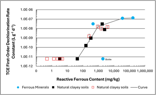
Figure 1: First-order rate constants for abiotic reductive dechlorination of TCE under anaerobic conditions. Circles are data from Schaefer
et al., 2021
[4], filled squares from Schaefer
et al., 2018
[5], and Schaefer
et al., 2017
[6], and open squares from Schaefer
et al., 2025
[1].
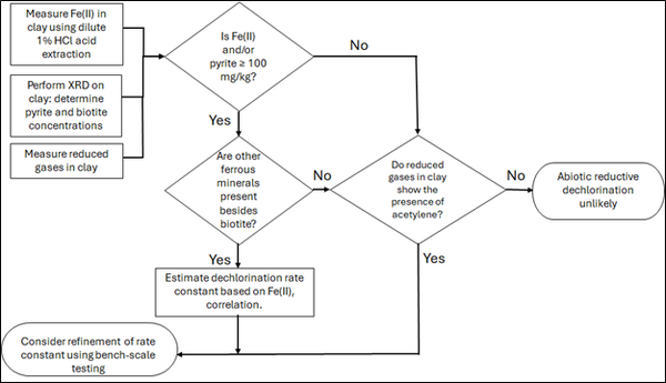
Figure 2: Flowchart diagram of field screening procedures
The recommended approach builds upon the methodology and findings of a recent study[1], emphasizing field-based and analytical techniques to quantify abiotic first-order reductive dechlorination rate constants for PCE and TCE in clayey soils under anoxic conditions. Key components of this evaluation are listed below:
- Zone Identification: The focus of the investigation should be to delineate clayey zones adjacent to hydraulically conductive zones.
- Ferrous Mineral Quantification: Assess ferrous mineral context in clay via 1% HCl extraction at ambient temperature over a 10-minute interval.
- Mineralogical Characterization: Conduct XRD analysis with the specific intent of identifying the presence of pyrite and biotite.
- Reduced Gas Analysis: Measurement of reduced gases such as acetylene, ethene, and ethane concentrations in clay samples. Gas-tight sampling devices (e.g., En Core® soil samplers by En Novative Technologies, Inc.) should be used to ensure sample integrity during collection and transport.
Clay samples should be collected within a few centimeters of the high-permeability interface, with optional additional sampling further inward. For mineralogical analysis, a defined interval may be collected and subsequently subsampled. To preserve sample integrity, exposure to air should be minimized during collection, transport, and handling. Homogenization should occur within an anaerobic chamber, and if subsamples are required for external analysis, they must be shipped in gas-tight, anaerobic containers.
Estimation of the abiotic reductive first-order rate constant for PCE and TCE is based on the “reactive” ferrous content in the clay. Reactive ferrous content (Fe(II)r) is estimated as shown in Equation 1:
- Equation 1: Fe(II)r = DA + XRDpyr - XRDbiotite
where DA is the ferrous content from the dilute acid (1% HCl) extraction, XRDpyr is the pyrite content from XRD analysis, and XRDbiotite is the biotite content from XRD analysis[1].
Abiotic dechlorination is unlikely to contribute to mitigating contaminant back-diffusion when reactive ferrous iron (Fe(II)r) concentrations are below 100 mg/kg (Figure 1). For Fe(II)r above 100 mg/kg, the first-order rate constant for PCE and TCE reductive dechlorination can be estimated using the correlation shown in Figure 1[5][7]. The rate constant exhibits a strong positive correlation with the logarithm of reactive Fe(II) content (Pearson’s r = 0.82), with a slope of 4.7 × 10⁻⁸ L g⁻¹ d⁻¹ (log mg kg⁻¹)⁻¹.
Figure 2 presents a decision flowchart designed to evaluate the significance and extent of abiotic reductive dechlorination. By applying Equation 1 to the dilute acid extractable Fe(II) plus measured mineral species data from clay samples, the reactive ferrous iron content (Fe(II)r) can be quantified, enabling a streamlined assessment of the extent to which abiotic processes are contributing to the mitigation of contaminant back-diffusion.
If Fe(II)r is ≥ 100 mg/kg, a first-order dechlorination rate constant can be estimated and subsequently used within a contaminant fate and transport model. However, if acetylene is detected in the clay, even with Fe(II)r less than 100 mg/kg, then bench-scale testing using methods similar to those described in a recent study[1] is recommended, as such results would likely be inconsistent with those shown in Figure 1, suggesting some other mechanism might be involved, or that the system mineralogy might be more complex than anticipated. Even if Fe(II)r ≥ 100 mg/kg, confirmatory bench-scale testing may be conducted for additional verification and to refine estimation of the abiotic dechlorination rate constant.
Summary and Recommendations
The approach outlined above is intended to serve as a generalized guide for practitioners and site managers to cost-effectively determine the extent to which beneficial abiotic reductive dechlorination reactions are likely occurring in low permeability (e.g., clayey) zones. This approach may be contraindicated if co-contaminants are present. It is currently unclear whether other classes of potentially reactive chemicals, such as trinitrotoluene (TNT) or chlorinated ethanes, could interact competitively with PCE and TCE.
In addition, it remains unclear how other classes of compounds such as per- and polyfluoroalkyl substances (PFAS) may interact or sorb with ferrous minerals and potentially inhibit abiotic dechlorination reactions. Coupling these recommended activities with conventional site investigation tasks would provide an opportunity to perform many of the up-front screening activities with minimal additional project costs. It is important to note that the guidance proposed herein pertains to particularly low permeability media. Sites with complex or varying lithology, where the mineralogy and/or redox conditions may vary, might require evaluation of multiple samples to provide appropriate site-wide information.
References
- ^ 1.0 1.1 1.2 1.3 1.4 Schaefer, C.E., Tran, D., Nguyen, D., Latta, D.E., Werth, C.J., 2025. Evaluating Mineral and In Situ Indicators of Abiotic Dechlorination in Clayey Soils. Groundwater Monitoring and Remediation, 45(2), pp. 31-39. doi: 10.1111/gwmr.12709
- ^ Falta, R., and Wang, W., 2017. A semi-analytical method for simulating matrix diffusion in numerical transport models. Journal of Contaminant Hydrology, 197, pp. 39-49. doi: 10.1016/j.jconhyd.2016.12.007 Open Access Manuscript
- ^ Kulkarni, P.R., Adamson, D.T., Popovic, J., Newell, C.J., 2022. Modeling a well-charactized perfluorooctane sulfate (PFOS) source and plume using the REMChlor-MD model to account for matrix diffusion. Journal of Contaminant Hydrology, 247, Article 103986. doi: 10.1016/j.jconhyd.2022.103986 Open Access Manuscript
- ^ Schaefer, C.E., Ho, P., Berns, E., Werth, C., 2021. Abiotic dechlorination in the presence of ferrous minerals. Journal of Contaminant Hydrology, 241, 103839. doi: 10.1016/j.jconhyd.2021.103839 Open Access Manuscript
- ^ 5.0 5.1 Schaefer, C.E., Ho, P., Berns, E., Werth, C., 2018. Mechanisms for abiotic dechlorination of trichloroethene by ferrous minerals under oxic and anoxic conditions in natural sediments. Environmental Science and Technology, 52(23), pp.13747-13755. doi: 10.1021/acs.est.8b04108
- ^ Schaefer, C.E., Ho., Gurr, C., Berns, E., Werth, C., 2017. Abiotic dechlorination of chlorinated ethenes in natural clayey soils: impacts of mineralogy and temperature. Journal of Contaminant Hydrology, 206, pp. 10-17. doi: 10.1016/j.jconhyd.2017.09.007 Open Access Manuscript
- ^ Borden, R.C., Cha, K.Y., 2021. Evaluating the impact of back diffusion on groundwater cleanup time. Journal of Contaminant Hydrology, 243, Article 103889. doi: 10.1016/j.jconhyd.2021 Open Access Manuscript
See Also

