|
|
| (816 intermediate revisions by the same user not shown) |
| Line 1: |
Line 1: |
| − | ==Hydrogeophysical methods for characterization and monitoring of surface water-groundwater interactions== | + | ==''In Situ'' Toxicity Identification Evaluation (iTIE)== |
| − | Hydrogeophysical methods can be used to cost-effectively locate and characterize regions of
| + | The ''in situ'' Toxicity Identification Evaluation system is a tool to incorporate in weight-of-evidence studies at sites with numerous chemical toxicant classes present. The technology works by continuously sampling site water, immediately fractionating the water using diagnostic sorptive resins, and then exposing test organisms to the water to observe toxicity responses with minimal sample manipulation. It is compatible with various resins, test organisms, and common acute and chronic toxicity tests, and can be deployed at sites with a wide variety of physical and logistical considerations. |
| − | enhanced groundwater/surface-water exchange (GWSWE) and to guide effective follow up investigations based on more traditional invasive methods. The most established methods exploit the contrasts in temperature and/or specific conductance that commonly exist between groundwater and surface water.
| |
| | <div style="float:right;margin:0 0 2em 2em;">__TOC__</div> | | <div style="float:right;margin:0 0 2em 2em;">__TOC__</div> |
| | | | |
| | '''Related Article(s):''' | | '''Related Article(s):''' |
| − | *[[Geophysical Methods]]
| |
| − | *[[Geophysical Methods - Case Studies]]
| |
| | | | |
| − | '''Contributor(s):'''
| + | *[[Contaminated Sediments - Introduction]] |
| − | *[[Dr. Lee Slater]] | + | *[[Contaminated Sediment Risk Assessment]] |
| − | *Dr. Ramona Iery | + | *[[Passive Sampling of Sediments]] |
| − | *Dr. Dimitrios Ntarlagiannis | + | *[[Sediment Porewater Dialysis Passive Samplers for Inorganics (Peepers)]] |
| − | *Henry Moore | |
| | | | |
| − | '''Key Resource(s):''' | + | '''Contributors:''' Dr. G. Allen Burton Jr., Austin Crane |
| − | *USGS Method Selection Tool: https://code.usgs.gov/water/espd/hgb/gw-sw-mst | + | |
| − | *USGS Water Resources: https://www.usgs.gov/mission-areas/water-resources/science/groundwatersurface-water-interaction | + | '''Key Resources:''' |
| | + | *A Novel In Situ Toxicity Identification Evaluation (iTIE) System for Determining which Chemicals Drive Impairments at Contaminated Sites<ref name="BurtonEtAl2020">Burton, G.A., Cervi, E.C., Meyer, K., Steigmeyer, A., Verhamme, E., Daley, J., Hudson, M., Colvin, M., Rosen, G., 2020. A novel In Situ Toxicity Identification Evaluation (iTIE) System for Determining which Chemicals Drive Impairments at Contaminated Sites. Environmental Toxicology and Chemistry, 39(9), pp. 1746-1754. [https://doi.org/10.1002/etc.4799 doi: 10.1002/etc.4799]</ref> |
| | + | *An in situ toxicity identification and evaluation water analysis system: Laboratory validation<ref name="SteigmeyerEtAl2017">Steigmeyer, A.J., Zhang, J., Daley, J.M., Zhang, X., Burton, G.A. Jr., 2017. An in situ toxicity identification and evaluation water analysis system: Laboratory validation. Environmental Toxicology and Chemistry, 36(6), pp. 1636-1643. [https://doi.org/10.1002/etc.3696 doi: 10.1002/etc.3696]</ref> |
| | + | *Sediment Toxicity Identification Evaluation (TIE) Phases I, II, and III Guidance Document<ref>United States Environmental Protection Agency, 2007. Sediment Toxicity Identification Evaluation (TIE) Phases I, II, and III Guidance Document, EPA/600/R-07/080. 145 pages. [https://nepis.epa.gov/Exe/ZyPURL.cgi?Dockey=P1003GR1.txt Free Download] [[Media: EPA2007.pdf | Report.pdf]]</ref> |
| | + | *In Situ Toxicity Identification Evaluation (iTIE) Technology for Assessing Contaminated Sediments, Remediation Success, Recontamination and Source Identification<ref>In Situ Toxicity Identification Evaluation (iTIE) Technology for Assessing Contaminated Sediments, Remediation Success, Recontamination and Source Identification [https://serdp-estcp.mil/projects/details/88a8f9ba-542b-4b98-bfa4-f693435535cd/er18-1181-project-overview Project Website] [[Media: ER18-1181Ph.II.pdf | Final Report.pdf]]</ref> |
| | | | |
| | ==Introduction== | | ==Introduction== |
| − | Discharges of contaminated groundwater to surface water bodies threaten ecosystems and degrade the quality of surface water resources. Subsurface heterogeneity associated with the geological setting and stratigraphy often results in such discharges occurring as localized zones (or seeps) of contaminated groundwater. Traditional methods for investigating GWSWE include [https://books.gw-project.org/groundwater-surface-water-exchange/chapter/seepage-meters/#:~:text=Seepage%20meters%20measure%20the%20flux,that%20it%20isolates%20water%20exchange. seepage meters]<ref>Rosenberry, D. O., Duque, C., and Lee, D. R., 2020. History and Evolution of Seepage Meters for Quantifying Flow between Groundwater and Surface Water: Part 1 – Freshwater Settings. Earth-Science Reviews, 204(103167). [https://doi.org/10.1016/j.earscirev.2020.103167 doi: 10.1016/j.earscirev.2020.103167].</ref><ref>Duque, C., Russoniello, C. J., and Rosenberry, D. O., 2020. History and Evolution of Seepage Meters for Quantifying Flow between Groundwater and Surface Water: Part 2 – Marine Settings and Submarine Groundwater Discharge. Earth-Science Reviews, 204 ( 103168). [https://doi.org/10.1016/j.earscirev.2020.103168 doi: 10.1016/j.earscirev.2020.103168].</ref>, which directly quantify the volume flux crossing the bed of a surface water body (i.e, a lake, river or wetland) and point probes that locally measure key water quality parameters (e.g., temperature, pore water velocity, specific conductance, dissolved oxygen, pH). Seepage meters provide direct estimates of seepage fluxes between groundwater and surface- water but are time consuming and can be difficult to deploy in high energy surface water environments and along armored bed sediments. Manual seepage meters rely on quantifying volume changes in a bag of water that is hydraulically connected to the bed. Although automated seepage meters such as the [https://clu-in.org/programs/21m2/navytools/gsw/#ultraseep Ultraseep system] have been developed, they are generally not suitable for long term deployment (weeks to months). The US Navy has developed the [https://clu-in.org/programs/21m2/navytools/gsw/#trident Trident probe] for more rapid (relative to seepage meters) sampling, whereby the probe is inserted into the bed and point-in-time pore water quality and sediment parameters are directly recorded (note that the Trident probe does not measure a seepage flux). Such direct probe-based measurements are still relatively time consuming to acquire, particularly when reconnaissance information is required over large areas to determine the location of discrete seeps for further, more quantitative analysis.
| + | In waterways impacted by numerous naturally occurring and anthropogenic chemical stressors, it is crucial for environmental practitioners to be able to identify which chemical classes are causing the highest degrees of toxicity to aquatic life. Previously developed methods, including the Toxicity Identification Evaluation (TIE) protocol developed by the US Environmental Protection Agency (EPA)<ref>Norberg-King, T., Mount, D.I., Amato, J.R., Jensen, D.A., Thompson, J.A., 1992. Toxicity identification evaluation: Characterization of chronically toxic effluents: Phase I. Publication No. EPA/600/6-91/005F. U.S. Environmental Protection Agency, Office of Research and Development. [https://www.epa.gov/sites/default/files/2015-09/documents/owm0255.pdf Free Download from US EPA] [[Media: usepa1992.pdf | Report.pdf]]</ref>, can be confounded by sample manipulation artifacts and temporal limitations of ''ex situ'' organism exposures<ref name="BurtonEtAl2020"/>. These factors may disrupt causal linkages and mislead investigators during site characterization and management decision-making. The ''in situ'' Toxicity Identification Evaluation (iTIE) technology was developed to allow users to strengthen stressor-causality linkages and rank chemical classes of concern at impaired sites, with high degrees of ecological realism. |
| | + | |
| | + | The technology has undergone a series of improvements in recent years, with the most recent prototype being robust, operable in a wide variety of site conditions, and cost-effective compared to alternative site characterization methods<ref>Burton, G.A. Jr., Nordstrom, J.F., 2004. An in situ toxicity identification evaluation method part I: Laboratory validation. Environmental Toxicology and Chemistry, 23(12), pp. 2844-2850. [https://doi.org/10.1897/03-409.1 doi: 10.1897/03-409.1]</ref><ref>Burton, G.A. Jr., Nordstrom, J.F., 2004. An in situ toxicity identification evaluation method part II: Field validation. Environmental Toxicology and Chemistry, 23(12), pp. 2851-2855. [https://doi.org/10.1897/03-468.1 doi: 10.1897/03-468.1]</ref><ref name="BurtonEtAl2020"/><ref name="SteigmeyerEtAl2017"/>. The latest prototype can be used in any of the following settings: in marine, estuarine, or freshwater sites; to study surface water or sediment pore water; in shallow waters easily accessible by foot or in deep waters only accessible by pier or boat. It can be used to study sites impacted by a wide variety of stressors including ammonia, [[Metal and Metalloid Contaminants | metals]], pesticides, polychlorinated biphenyls (PCB), [[Polycyclic Aromatic Hydrocarbons (PAHs) | polycyclic aromatic hydrocarbons (PAH)]], and [[Perfluoroalkyl and Polyfluoroalkyl Substances (PFAS) | per- and polyfluoroalkyl substances (PFAS)]], among others. The technology is applicable to studies of acute toxicity via organism survival or of chronic toxicity via responses in growth, reproduction, or gene expression<ref name="BurtonEtAl2020"/>. |
| | + | |
| | + | ==System Components and Validation== |
| | + | [[File: CraneFig1.png | thumb | 600 px | Figure 1: A schematic diagram of the iTIE system prototype. The system is divided into three sub-systems: 1) the Pore Water/Surface Water Collection Sub-System (blue); 2) the Pumping Sub-System (red); and 3) the iTIE Resin, Exposure, and Sampling Sub-System (green). Water first enters the system through the Pore Water/Surface Water Collection Sub-System. Porewater can be collected using Trident-style probes, or surface water can be collected using a simple weighted probe. The water is composited in a manifold before being pumped to the rest of the iTIE system by the booster pump. Once in the iTIE Resin, Exposure, and Sampling Sub-System, the water is gently oxygenated by the Oxygen Coil, separated from gas bubbles by the Drip Chamber, and diverted to separate iTIE Resin and Exposure Chambers (or iTIE units) by the Splitting Manifold. Water movement through each iTIE unit is controlled by a dedicated Regulation Pump. Finally, the water is gathered in Sample Collection bottles for analysis.]] |
| | + | The latest iTIE prototype consists of an array of sorptive resins that differentially fractionate sampled water, and a series of corresponding flow-through organism chambers that receive the treated water ''in situ''. Resin treatments can be selected depending on the chemicals suspected to be present at each site to selectively sequester certain chemical of concern (CoC) classes from the whole water, leaving a smaller subset of chemicals in the resulting water fraction for chemical and toxicological characterization. Test organism species and life stages can also be chosen depending on factors including site characteristics and study goals. In the full iTIE protocol, site water is continuously sampled either from the sediment pore spaces or the water column at a site, gently oxygenated, diverted to different iTIE units for fractionation and organism exposure, and collected in sample bottles for off-site chemical analysis (Figure 1). All iTIE system components are housed within waterproof Pelican cases, which allow for ease of transport and temperature control. |
| | + | |
| | + | ===Porewater and Surface Water Collection Sub-system=== |
| | + | [[File: CraneFig2.png | thumb | 600 px | Figure 2: a) Trident probe with auxiliary sensors attached, b) a Trident probe with end caps removed (the red arrow identifies the intermediate space where glass beads are packed to filter suspended solids), c) a Trident probe being installed using a series of push poles and a fence post driver]] |
| | + | Given the importance of sediment porewater to ecosystem structure and function, investigators may employ the iTIE system to evaluate the toxic effects associated with the impacted sediment porewater. To accomplish this, the iTIE system utilizes the Trident probe, originally developed for Department of Defense site characterization studies<ref>Chadwick, D.B., Harre, B., Smith, C.F., Groves, J.G., Paulsen, R.J., 2003. Coastal Contaminant Migration Monitoring: The Trident Probe and UltraSeep System. Hardware Description, Protocols, and Procedures. Technical Report 1902. Space and Naval Warfare Systems Center.</ref>. The main body of the Trident is comprised of a stainless-steel frame with six hollow probes (Figure 2). Each probe contains a layer of inert glass beads, which filters suspended solids from the sampled water. The water is drawn through each probe into a composite manifold and transported to the rest of the iTIE system using a high-precision peristaltic pump. |
| | + | |
| | + | The Trident also includes an adjustable stopper plate, which forms a seal against the sediment and prevents the inadvertent dilution of porewater samples with surface water. (Figure 2). Preliminary laboratory results indicate that the Trident is extremely effective in collecting porewater samples with minimal surface water infiltration in sediments ranging from coarse sand to fine clay. Underwater cameras, sensors, passive samplers, and other auxiliary equipment can be attached to the Trident probe frame to provide supplemental data. |
| | + | |
| | + | Alternatively, practitioners may employ the iTIE system to evaluate site surface water. To sample surface water, weighted intake tubes can collect surface water from the water column using a peristaltic pump. |
| | + | |
| | + | ===Oxygen Coil, Overflow Bag and Drip Chamber=== |
| | + | [[File: CraneFig3.png | thumb | left | 400 px | Figure 3. Contents of the iTIE system cooler. The pictured HDPE rack (47.6 cm length x 29.7 cm width x 33.7 cm height) is removable from the iTIE cooler. Water enters the system at the red circle, flows through the oxygen coil, and then travels to each of the individual iTIE units where diagnostic resins and organisms are located. The water then briefly leaves the cooler to travel through peristaltic regulation pumps before being gathered in sample collection bottles.]] |
| | + | Porewater is naturally anoxic due to limited mixing with aerated surface water and high oxygen demand of sediments, which may cause organism mortality and interfere with iTIE results. To preclude this, sampled porewater is exposed to an oxygen coil. This consists of an interior silicone tube connected to a pressurized oxygen canister, threaded through an exterior reinforced PVC tube through which water is slowly pumped (Figure 3). Pump rates are optimized to ensure adequate aeration of the water. In addition to elevating DO levels, the oxygen coil facilitates the oxidation of dissolved sulfides, which naturally occur in some marine sediments and may otherwise cause toxicity to organisms if left in its reduced form. |
| | | | |
| − | Over the last few decades, a broader toolbox of hydrogeophysical technologies has been developed to rapidly and non-invasively evaluate zones of GWSWE in a variety of surface water settings, spanning from freshwater bodies to saline coastal environments. Many of these technologies are currently being deployed under a Department of Defense Environmental Security Technology Certification Program ([https://serdp-estcp.mil/ ESTCP]) project ([https://serdp-estcp.mil/projects/details/e4a12396-4b56-4318-b9e5-143c3011b8ff ER21-5237]) to demonstrate the value of the toolbox to remedial program managers (RPMs) dealing with the challenge of characterizing surface water contamination via groundwater from facilities proximal to surface water bodies. This article summarizes these technologies and provides references to key resources, mostly provided by the [https://www.usgs.gov/mission-areas/water-resources Water Resources Mission Area] of the United States Geological Survey that describe the technologies in further detail.
| + | Gas bubbles may form in the oxygen coil over the course of a deployment. These can be disruptive, decreasing water sample volumes and posing a danger to sensitive organisms like daphnids. To account for this, the water travels to a drip chamber after exiting the oxygen coil, which allows gas bubbles to be separated and diverted to an overflow system. The sample water then flows to a manifold which divides the flow into different paths to each of the treatment units for fractionation and organism exposure. |
| | | | |
| − | ==Hydrogeophysical Technologies for Understanding Groundwater-Surface Water Interactions== | + | ===iTIE Units: Fractionation and Organism Exposure Chambers=== |
| − | [[Wikipedia: Hydrogeophysics |Hydrogeophysical technologies]] exploit contrasts in the physical properties between groundwater and surface water to detect and monitor zones of pronounced GWSWE. The two most valuable properties to measure are temperature and electrical conductivity. Temperature has been used for decades as an indicator of groundwater-surface water exchange | + | [[File: CraneFig4.png | thumb | 300px | Figure 4. A diagram of the iTIE prototype. Water flows upward into each resin chamber through the unit bottom. After being chemically fractionated in the resin chamber, water travels into the organism chamber, where test organisms have been placed. Water is drawn through the units by high-precision peristaltic pumps.]] |
| | + | At the core of the iTIE system are separate dual-chamber iTIE units, each with a resin fractionation chamber and an organism exposure chamber (Figure 4). Developed by Burton ''et al.''<ref name="BurtonEtAl2020"/>, the iTIE prototype is constructed from acrylic, with rubber O-rings to connect each piece. Each iTIE unit can contain a different diagnostic resin matrix, customizable to remove specific chemical classes from the water. Sampled water flows into each unit through the bottom and is differentially fractionated by the resin matrix as it travels upward. Then it reaches the organism chamber, where test organisms are placed for exposure. The organism chamber inlet and outlet are covered by mesh to prevent the escape of the test organisms. This continuous flow-through design allows practitioners to capture the temporal heterogeneity of ambient water conditions over the duration of an ''in situ'' exposure. Currently, the iTIE system can support four independent iTIE treatment units. |
| | | | |
| − | [[File:AbioMCredFig4.png | thumb |600px|Figure 4. Chemical structure of commonly used hydroquinones in NACs/MCs kinetic experiments.]]
| + | After being exposed to test organisms, water is collected in sample bottles. The bottles can be pre-loaded with preservation reagents to allow for later chemical analysis. Sample bottles can be composed of polyethylene, glass or other materials depending on the CoC. |
| − | The two most predominant forms of organic carbon in natural systems are natural organic matter (NOM) and black carbon (BC)<ref name="Schumacher2002">Schumacher, B.A., 2002. Methods for the Determination of Total Organic Carbon (TOC) in Soils and Sediments. U.S. EPA, Ecological Risk Assessment Support Center. [http://bcodata.whoi.edu/LaurentianGreatLakes_Chemistry/bs116.pdf Free download.]</ref>. Black carbon includes charcoal, soot, graphite, and coal. Until the early 2000s black carbon was considered to be a class of (bio)chemically inert geosorbents<ref name="Schmidt2000">Schmidt, M.W.I., and Noack, A.G., 2000. Black carbon in soils and sediments: Analysis, distribution, implications, and current challenges. Global Biogeochemical Cycles, 14(3), pp. 777–793. [https://doi.org/10.1029/1999GB001208 DOI: 10.1029/1999GB001208] [https://agupubs.onlinelibrary.wiley.com/doi/epdf/10.1029/1999GB001208 Open access article.]</ref>. However, it has been shown that BC can contain abundant quinone functional groups and thus can store and exchange electrons<ref name="Klüpfel2014">Klüpfel, L., Keiluweit, M., Kleber, M., and Sander, M., 2014. Redox Properties of Plant Biomass-Derived Black Carbon (Biochar). Environmental Science and Technology, 48(10), pp. 5601–5611. [https://doi.org/10.1021/es500906d DOI: 10.1021/es500906d]</ref> with chemical<ref name="Xin2019">Xin, D., Xian, M., and Chiu, P.C., 2019. New methods for assessing electron storage capacity and redox reversibility of biochar. Chemosphere, 215, 827–834. [https://doi.org/10.1016/j.chemosphere.2018.10.080 DOI: 10.1016/j.chemosphere.2018.10.080]</ref> and biological<ref name="Saquing2016">Saquing, J.M., Yu, Y.-H., and Chiu, P.C., 2016. Wood-Derived Black Carbon (Biochar) as a Microbial Electron Donor and Acceptor. Environmental Science and Technology Letters, 3(2), pp. 62–66. [https://doi.org/10.1021/acs.estlett.5b00354 DOI: 10.1021/acs.estlett.5b00354]</ref> agents in the surroundings. Specifically, BC such as biochar has been shown to reductively transform MCs including NTO, DNAN, and RDX<ref name="Xin2022"/>.
| |
| | | | |
| − | NOM encompasses all the organic compounds present in terrestrial and aquatic environments and can be classified into two groups, non-humic and humic substances. Humic substances (HS) contain a wide array of functional groups including carboxyl, enol, ether, ketone, ester, amide, (hydro)quinone, and phenol<ref name="Sparks2003">Sparks, D.L., 2003. Environmental Soil Chemistry, 2nd Edition. Elsevier Science and Technology Books. [https://doi.org/10.1016/B978-0-12-656446-4.X5000-2 DOI: 10.1016/B978-0-12-656446-4.X5000-2]</ref>. Quinone and hydroquinone groups are believed to be the predominant redox moieties responsible for the capacity of HS and BC to store and reversibly accept and donate electrons (i.e., through reduction and oxidation of HS/BC, respectively)<ref name="Schwarzenbach1990"/><ref name="Dunnivant1992"/><ref name="Klüpfel2014"/><ref name="Scott1998">Scott, D.T., McKnight, D.M., Blunt-Harris, E.L., Kolesar, S.E., and Lovley, D.R., 1998. Quinone Moieties Act as Electron Acceptors in the Reduction of Humic Substances by Humics-Reducing Microorganisms. Environmental Science and Technology, 32(19), pp. 2984–2989. [https://doi.org/10.1021/es980272q DOI: 10.1021/es980272q]</ref><ref name="Cory2005">Cory, R.M., and McKnight, D.M., 2005. Fluorescence Spectroscopy Reveals Ubiquitous Presence of Oxidized and Reduced Quinones in Dissolved Organic Matter. Environmental Science & Technology, 39(21), pp 8142–8149. [https://doi.org/10.1021/es0506962 DOI: 10.1021/es0506962]</ref><ref name="Fimmen2007">Fimmen, R.L., Cory, R.M., Chin, Y.P., Trouts, T.D., and McKnight, D.M., 2007. Probing the oxidation–reduction properties of terrestrially and microbially derived dissolved organic matter. Geochimica et Cosmochimica Acta, 71(12), pp. 3003–3015. [https://doi.org/10.1016/j.gca.2007.04.009 DOI: 10.1016/j.gca.2007.04.009]</ref><ref name="Struyk2001">Struyk, Z., and Sposito, G., 2001. Redox properties of standard humic acids. Geoderma, 102(3-4), pp. 329–346. [https://doi.org/10.1016/S0016-7061(01)00040-4 DOI: 10.1016/S0016-7061(01)00040-4]</ref><ref name="Ratasuk2007">Ratasuk, N., and Nanny, M.A., 2007. Characterization and Quantification of Reversible Redox Sites in Humic Substances. Environmental Science and Technology, 41(22), pp. 7844–7850. [https://doi.org/10.1021/es071389u DOI: 10.1021/es071389u]</ref><ref name="Aeschbacher2010">Aeschbacher, M., Sander, M., and Schwarzenbach, R.P., 2010. Novel Electrochemical Approach to Assess the Redox Properties of Humic Substances. Environmental Science and Technology, 44(1), pp. 87–93. [https://doi.org/10.1021/es902627p DOI: 10.1021/es902627p]</ref><ref name="Aeschbacher2011">Aeschbacher, M., Vergari, D., Schwarzenbach, R.P., and Sander, M., 2011. Electrochemical Analysis of Proton and Electron Transfer Equilibria of the Reducible Moieties in Humic Acids. Environmental Science and Technology, 45(19), pp. 8385–8394. [https://doi.org/10.1021/es201981g DOI: 10.1021/es201981g]</ref><ref name="Bauer2009">Bauer, I., and Kappler, A., 2009. Rates and Extent of Reduction of Fe(III) Compounds and O<sub>2</sub> by Humic Substances. Environmental Science and Technology, 43(13), pp. 4902–4908. [https://doi.org/10.1021/es900179s DOI: 10.1021/es900179s]</ref><ref name="Maurer2010">Maurer, F., Christl, I. and Kretzschmar, R., 2010. Reduction and Reoxidation of Humic Acid: Influence on Spectroscopic Properties and Proton Binding. Environmental Science and Technology, 44(15), pp. 5787–5792. [https://doi.org/10.1021/es100594t DOI: 10.1021/es100594t]</ref><ref name="Walpen2016">Walpen, N., Schroth, M.H., and Sander, M., 2016. Quantification of Phenolic Antioxidant Moieties in Dissolved Organic Matter by Flow-Injection Analysis with Electrochemical Detection. Environmental Science and Technology, 50(12), pp. 6423–6432. [https://doi.org/10.1021/acs.est.6b01120 DOI: 10.1021/acs.est.6b01120] [https://pubs.acs.org/doi/pdf/10.1021/acs.est.6b01120 Open access article.]</ref><ref name="Aeschbacher2012">Aeschbacher, M., Graf, C., Schwarzenbach, R.P., and Sander, M., 2012. Antioxidant Properties of Humic Substances. Environmental Science and Technology, 46(9), pp. 4916–4925. [https://doi.org/10.1021/es300039h DOI: 10.1021/es300039h]</ref><ref name="Nurmi2002">Nurmi, J.T., and Tratnyek, P.G., 2002. Electrochemical Properties of Natural Organic Matter (NOM), Fractions of NOM, and Model Biogeochemical Electron Shuttles. Environmental Science and Technology, 36(4), pp. 617–624. [https://doi.org/10.1021/es0110731 DOI: 10.1021/es0110731]</ref>.
| + | ===Pumping Sub-system=== |
| | + | [[File: CraneFig5.png | thumb | 300px | Figure 5. The iTIE system pumping sub-system. The sub-system consists of: A) a single booster pump, which is directly connected to the water sampling device and feeds water to the rest of the iTIE system, and B) a set of four regulation pumps, which each connect to the outflow of an individual iTIE unit. Each pump set is housed in a waterproof case with self-contained rechargeable battery power. A tablet is mounted inside the lid of the four pump case, which can be used to program and operate all of the pumps when connected to the internet.]] |
| | + | Water movement through the system is driven by a series of high-precision, programmable peristaltic pumps ([https://ecotechmarine.com/ EcoTech Marine]). Each pump set is housed in a Pelican storm travel case. Power is supplied to each pump by internal rechargeable lithium-iron phosphate batteries ([https://www.bioennopower.com/ Bioenno Power]). |
| | | | |
| − | Hydroquinones have been widely used as surrogates to understand the reductive transformation of NACs and MCs by NOM. Figure 4 shows the chemical structures of the singly deprotonated forms of four hydroquinone species previously used to study NAC/MC reduction. The second-order rate constants (''k<sub>R</sub>'') for the reduction of NACs/MCs by these hydroquinone species are listed in Table 1, along with the aqueous-phase one electron reduction potentials of the NACs/MCs (''E<sub>H</sub><sup>1’</sup>'') where available. ''E<sub>H</sub><sup>1’</sup>'' is an experimentally measurable thermodynamic property that reflects the propensity of a given NAC/MC to accept an electron in water (''E<sub>H</sub><sup>1</sup>''(R-NO<sub>2</sub>)):
| + | First, water is supplied to the system by a booster pump (Figure 5A). This pump is situated between the water sampling sub-system and the oxygen coil. The booster pump: 1) facilitates pore water collection, especially from sediments with high fine particle fractions; 2) helps water overcome vertical lifts to travel to the iTIE system; and 3) prevents vacuums from forming in the iTIE system interior, which can accelerate the formation of disruptive gas bubbles in the oxygen coil. The booster pump should be programmed to supply an excess of water to prevent vacuum formation. |
| | | | |
| − | :::::<big>'''Equation 1:''' ''R-NO<sub>2</sub> + e<sup>-</sup> ⇔ R-NO<sub>2</sub><sup>•-</sup>''</big>
| + | Second, a set of four regulation pumps ensure precise flow rates through each independent iTIE unit (Figure 5B). Each regulation pump pulls water from the top of an iTIE unit and then dispenses that water into a sample bottle for further analysis. |
| | | | |
| − | Knowing the identity of and reaction order in the reductant is required to derive the second-order rate constants listed in Table 1. This same reason limits the utility of reduction rate constants measured with complex carbonaceous reductants such as NOM<ref name="Dunnivant1992"/>, BC<ref name="Oh2013"/><ref name="Oh2009"/><ref name="Xu2015"/><ref name="Xin2021">Xin, D., 2021. Understanding the Electron Storage Capacity of Pyrogenic Black Carbon: Origin, Redox Reversibility, Spatial Distribution, and Environmental Applications. Doctoral Thesis, University of Delaware. [https://udspace.udel.edu/bitstream/handle/19716/30105/Xin_udel_0060D_14728.pdf?sequence=1 Free download.]</ref>, and HS<ref name="Luan2010"/><ref name="Murillo-Gelvez2021"/>, whose chemical structures and redox moieties responsible for the reduction, as well as their abundance, are not clearly defined or known. In other words, the observed rate constants in those studies are specific to the experimental conditions (e.g., pH and NOM source and concentration), and may not be easily comparable to other studies.
| + | ==Study Design Considerations== |
| | + | ===Diagnostic Resin Treatments=== |
| | + | Several commercially available resins have been verified for use in the iTIE system. Investigators can select resins based on stressor classes of interest at each site. Each resin selectively removes a CoC class from site water prior to organism exposure. |
| | + | *[https://www.dupont.com/products/ambersorb560.html DuPont Ambersorb 560] for removal of 1,4-dioxane and other organic chemicals<ref>Woodard, S., Mohr, T., Nickelsen, M.G., 2014. Synthetic media: A promising new treatment technology for 1,4-dioxane. Remediation Journal, 24(4), pp. 27-40. [https://doi.org/10.1002/rem.21402 doi: 10.1002/rem.21402]</ref> |
| | + | *C18 for nonpolar organic chemicals |
| | + | *[https://www.bio-rad.com/en-us Bio-Rad] [https://www.bio-rad.com/en-us/product/chelex-100-resin?ID=6448ab3e-b96a-4162-9124-7b7d2330288e Chelex] for metals |
| | + | *Granular activated carbon for metals, general organic chemicals, sulfide<ref>Lemos, B.R.S., Teixeira, I.F., de Mesquita, J.P., Ribeiro, R.R., Donnici, C.L., Lago, R.M., 2012. Use of modified activated carbon for the oxidation of aqueous sulfide. Carbon, 50(3), pp. 1386-1393. [https://doi.org/10.1016/j.carbon.2011.11.011 doi: 10.1016/j.carbon.2011.11.011]</ref> |
| | + | *[https://www.waters.com/nextgen/us/en.html Waters] [https://www.waters.com/nextgen/us/en/search.html?category=Shop&isocode=en_US&keyword=oasis%20hlb&multiselect=true&page=1&rows=12&sort=best-sellers&xcid=ppc-ppc_23916&gad_source=1&gad_campaignid=14746094146&gbraid=0AAAAAD_uR00nhlNwrhhegNh06pBODTgiN&gclid=CjwKCAiAtLvMBhB_EiwA1u6_PsppE0raci2IhvGnAAe5ijciNcetLaGZo5qA3g3r4Z_La7YAPJtzShoC6LoQAvD_BwE Oasis HLB] for general organic chemicals<ref name="SteigmeyerEtAl2017"/> |
| | + | *[https://www.waters.com/nextgen/us/en.html Waters] [https://www.waters.com/nextgen/us/en/search.html?category=All&enableHL=true&isocode=en_US&keyword=Oasis%20WAX%20&multiselect=true&page=1&rows=12&sort=most-relevant Oasis WAX] for PFAS, organic chemicals of mixed polarity<ref>Iannone, A., Carriera, F., Di Fiore, C., Avino, P., 2024. Poly- and Perfluoroalkyl Substance (PFAS) Analysis in Environmental Matrices: An Overview of the Extraction and Chromatographic Detection Methods. Analytica, 5(2), pp. 187-202. [https://doi.org/10.3390/analytica5020012 doi: 10.3390/analytica5020012] [[Media: IannoneEtAl2024.pdf | Open Access Article]]</ref> |
| | + | *Zeolite for ammonia, other organic chemicals |
| | | | |
| − | {| class="wikitable mw-collapsible" style="float:left; margin-right:40px; text-align:center;"
| + | Resins must be adequately conditioned prior to use. Otherwise, they may inadequately adsorb toxicants or cause stress to organisms. New resins should be tested for efficacy and toxicity before being used in an iTIE system. |
| − | |+ Table 1. Aqueous phase one electron reduction potentials and logarithm of second-order rate constants for the reduction of NACs and MCs by the singly deprotonated form of the hydroquinones lawsone, juglone, AHQDS and AHQS, with the second-order rate constants for the deprotonated NAC/MC species (i.e., nitrophenolates and NTO<sup>–</sup>) in parentheses.
| |
| − | |-
| |
| − | ! Compound
| |
| − | ! rowspan="2" |''E<sub>H</sub><sup>1'</sup>'' (V)
| |
| − | ! colspan="4"| Hydroquinone [log ''k<sub>R</sub>'' (M<sup>-1</sup>s<sup>-1</sup>)]
| |
| − | |-
| |
| − | ! (NAC/MC)
| |
| − | ! LAW<sup>-</sup>
| |
| − | ! JUG<sup>-</sup>
| |
| − | ! AHQDS<sup>-</sup>
| |
| − | ! AHQS<sup>-</sup>
| |
| − | |-
| |
| − | | Nitrobenzene (NB) || -0.485<ref name="Schwarzenbach1990"/> || 0.380<ref name="Schwarzenbach1990"/> || -1.102<ref name="Schwarzenbach1990"/> || 2.050<ref name="Murillo-Gelvez2019"/> || 3.060<ref name="Murillo-Gelvez2019"/>
| |
| − | |-
| |
| − | | 2-nitrotoluene (2-NT) || -0.590<ref name="Schwarzenbach1990"/> || -1.432<ref name="Schwarzenbach1990"/> || -2.523<ref name="Schwarzenbach1990"/> || 0.775<ref name="Hartenbach2008"/> ||
| |
| − | |-
| |
| − | | 3-nitrotoluene (3-NT) || -0.475<ref name="Schwarzenbach1990"/> || 0.462<ref name="Schwarzenbach1990"/> || -0.921<ref name="Schwarzenbach1990"/> || ||
| |
| − | |-
| |
| − | | 4-nitrotoluene (4-NT) || -0.500<ref name="Schwarzenbach1990"/> || 0.041<ref name="Schwarzenbach1990"/> || -1.292<ref name="Schwarzenbach1990"/> || 1.822<ref name="Hartenbach2008"/> || 2.610<ref name="Murillo-Gelvez2019"/>
| |
| − | |-
| |
| − | | 2-chloronitrobenzene (2-ClNB) || -0.485<ref name="Schwarzenbach1990"/> || 0.342<ref name="Schwarzenbach1990"/> || -0.824<ref name="Schwarzenbach1990"/> ||2.412<ref name="Hartenbach2008"/> ||
| |
| − | |-
| |
| − | | 3-chloronitrobenzene (3-ClNB) || -0.405<ref name="Schwarzenbach1990"/> || 1.491<ref name="Schwarzenbach1990"/> || 0.114<ref name="Schwarzenbach1990"/> || ||
| |
| − | |-
| |
| − | | 4-chloronitrobenzene (4-ClNB) || -0.450<ref name="Schwarzenbach1990"/> || 1.041<ref name="Schwarzenbach1990"/> || -0.301<ref name="Schwarzenbach1990"/> || 2.988<ref name="Hartenbach2008"/> ||
| |
| − | |-
| |
| − | | 2-acetylnitrobenzene (2-AcNB) || -0.470<ref name="Schwarzenbach1990"/> || 0.519<ref name="Schwarzenbach1990"/> || -0.456<ref name="Schwarzenbach1990"/> || ||
| |
| − | |-
| |
| − | | 3-acetylnitrobenzene (3-AcNB) || -0.405<ref name="Schwarzenbach1990"/> || 1.663<ref name="Schwarzenbach1990"/> || 0.398<ref name="Schwarzenbach1990"/> || ||
| |
| − | |-
| |
| − | | 4-acetylnitrobenzene (4-AcNB) || -0.360<ref name="Schwarzenbach1990"/> || 2.519<ref name="Schwarzenbach1990"/> || 1.477<ref name="Schwarzenbach1990"/> || ||
| |
| − | |-
| |
| − | | 2-nitrophenol (2-NP) || || 0.568 (0.079)<ref name="Schwarzenbach1990"/> || || ||
| |
| − | |-
| |
| − | | 4-nitrophenol (4-NP) || || -0.699 (-1.301)<ref name="Schwarzenbach1990"/> || || ||
| |
| − | |-
| |
| − | | 4-methyl-2-nitrophenol (4-Me-2-NP) || || 0.748 (0.176)<ref name="Schwarzenbach1990"/> || || ||
| |
| − | |-
| |
| − | | 4-chloro-2-nitrophenol (4-Cl-2-NP) || || 1.602 (1.114)<ref name="Schwarzenbach1990"/> || || ||
| |
| − | |-
| |
| − | | 5-fluoro-2-nitrophenol (5-Cl-2-NP) || || 0.447 (-0.155)<ref name="Schwarzenbach1990"/> || || ||
| |
| − | |-
| |
| − | | 2,4,6-trinitrotoluene (TNT) || -0.280<ref name="Schwarzenbach2016"/> || || 2.869<ref name="Hofstetter1999"/> || 5.204<ref name="Hartenbach2008"/> ||
| |
| − | |-
| |
| − | | 2-amino-4,6-dinitrotoluene (2-A-4,6-DNT) || -0.400<ref name="Schwarzenbach2016"/> || || 0.987<ref name="Hofstetter1999"/> || ||
| |
| − | |-
| |
| − | | 4-amino-2,6-dinitrotoluene (4-A-2,6-DNT) || -0.440<ref name="Schwarzenbach2016"/> || || 0.079<ref name="Hofstetter1999"/> || ||
| |
| − | |-
| |
| − | | 2,4-diamino-6-nitrotoluene (2,4-DA-6-NT) || -0.505<ref name="Schwarzenbach2016"/> || || -1.678<ref name="Hofstetter1999"/> || ||
| |
| − | |-
| |
| − | | 2,6-diamino-4-nitrotoluene (2,6-DA-4-NT) || -0.495<ref name="Schwarzenbach2016"/> || || -1.252<ref name="Hofstetter1999"/> || ||
| |
| − | |-
| |
| − | | 1,3-dinitrobenzene (1,3-DNB) || -0.345<ref name="Hofstetter1999"/> || || 1.785<ref name="Hofstetter1999"/> || ||
| |
| − | |-
| |
| − | | 1,4-dinitrobenzene (1,4-DNB) || -0.257<ref name="Hofstetter1999"/> || || 3.839<ref name="Hofstetter1999"/> || ||
| |
| − | |-
| |
| − | | 2-nitroaniline (2-NANE) || < -0.560<ref name="Hofstetter1999"/> || || -2.638<ref name="Hofstetter1999"/> || ||
| |
| − | |-
| |
| − | | 3-nitroaniline (3-NANE) || -0.500<ref name="Hofstetter1999"/> || || -1.367<ref name="Hofstetter1999"/> || ||
| |
| − | |-
| |
| − | | 1,2-dinitrobenzene (1,2-DNB) || -0.290<ref name="Hofstetter1999"/> || || || 5.407<ref name="Hartenbach2008"/> ||
| |
| − | |-
| |
| − | | 4-nitroanisole (4-NAN) || || -0.661<ref name="Murillo-Gelvez2019"/> || || 1.220<ref name="Murillo-Gelvez2019"/> ||
| |
| − | |-
| |
| − | | 2-amino-4-nitroanisole (2-A-4-NAN) || || -0.924<ref name="Murillo-Gelvez2019"/> || || 1.150<ref name="Murillo-Gelvez2019"/> || 2.190<ref name="Murillo-Gelvez2019"/>
| |
| − | |-
| |
| − | | 4-amino-2-nitroanisole (4-A-2-NAN) || || || ||1.610<ref name="Murillo-Gelvez2019"/> || 2.360<ref name="Murillo-Gelvez2019"/>
| |
| − | |-
| |
| − | | 2-chloro-4-nitroaniline (2-Cl-5-NANE) || || -0.863<ref name="Murillo-Gelvez2019"/> || || 1.250<ref name="Murillo-Gelvez2019"/> || 2.210<ref name="Murillo-Gelvez2019"/>
| |
| − | |-
| |
| − | | N-methyl-4-nitroaniline (MNA) || || -1.740<ref name="Murillo-Gelvez2019"/> || || -0.260<ref name="Murillo-Gelvez2019"/> || 0.692<ref name="Murillo-Gelvez2019"/>
| |
| − | |-
| |
| − | | 3-nitro-1,2,4-triazol-5-one (NTO) || || || || 5.701 (1.914)<ref name="Murillo-Gelvez2021"/> ||
| |
| − | |-
| |
| − | | Hexahydro-1,3,5-trinitro-1,3,5-triazine (RDX) || || || || -0.349<ref name="Kwon2008"/> ||
| |
| − | |}
| |
| | | | |
| − | [[File:AbioMCredFig5.png | thumb |500px|Figure 5. Relative reduction rate constants of the NACs/MCs listed in Table 1 for AHQDS<sup>–</sup>. Rate constants are compared with respect to RDX. Abbreviations of NACs/MCs as listed in Table 1.]]
| + | ===Test Organism Species and Life Stages=== |
| − | Most of the current knowledge about MC degradation is derived from studies using NACs. The reduction kinetics of only four MCs, namely TNT, N-methyl-4-nitroaniline (MNA), NTO, and RDX, have been investigated with hydroquinones. Of these four MCs, only the reduction rates of MNA and TNT have been modeled<ref name="Hofstetter1999"/><ref name="Murillo-Gelvez2019"/><ref name="Riefler2000">Riefler, R.G., and Smets, B.F., 2000. Enzymatic Reduction of 2,4,6-Trinitrotoluene and Related Nitroarenes: Kinetics Linked to One-Electron Redox Potentials. Environmental Science and Technology, 34(18), pp. 3900–3906. [https://doi.org/10.1021/es991422f DOI: 10.1021/es991422f]</ref><ref name="Salter-Blanc2015">Salter-Blanc, A.J., Bylaska, E.J., Johnston, H.J., and Tratnyek, P.G., 2015. Predicting Reduction Rates of Energetic Nitroaromatic Compounds Using Calculated One-Electron Reduction Potentials. Environmental Science and Technology, 49(6), pp. 3778–3786. [https://doi.org/10.1021/es505092s DOI: 10.1021/es505092s] [https://pubs.acs.org/doi/pdf/10.1021/es505092s Open access article.]</ref>.
| + | Practitioners can also select different organism species and life stages for use in the iTIE system, depending on site characteristics and study goals. The iTIE system can accommodate various small test organisms, including embryo-stage fish and most macroinvertebrates. The following common toxicity tests can be adapted for application within iTIE systems<ref>U.S. Environmental Protection Agency, Office of Solid Waste and Emergency Response, 1994. Catalogue of Standard Toxicity Tests for Ecological Risk Assessment. ECO Update, 2(2), 4 pages. Publication No. 9345.0.05I [https://www.epa.gov/sites/default/files/2015-09/documents/v2no2.pdf Free Download] [[Media: usepa1994.pdf | Report.pdf]]</ref>. |
| | + | <ul><u>Freshwater acute toxicity:</u></ul> |
| | + | *[[Wikipedia: Daphnia magna | ''Daphnia magna'']] or [[Wikipedia: Daphnia pulex | ''Daphnia pulex'']] 24-, 48-, and 96-hour survival |
| | + | <ul><u>Freshwater chronic toxicity:</u></ul> |
| | + | *[[Wikipedia: Ceriodaphnia dubia | ''Ceriodaphnia dubia'']] 7-day survival and reproduction |
| | + | *''D. magna'' 7-day survival and reproduction |
| | + | *[[Wikipedia: Fathead minnow | ''Pimephales promelas'']] 7-day embryo-larval survival and teratogenicity |
| | + | *[[Wikipedia: Hyalella azteca | ''Hyalella Azteca'']] 10- or 30-day survival and reproduction |
| | + | <ul><u>Marine acute toxicity:</u></ul> |
| | + | *[[Wikipedia: Americamysis bahia | ''Americamysis bahia'']] 24- and 48-hour survival |
| | + | <ul><u>Marine chronic toxicity:</u></ul> |
| | + | *''Americamysis'' survival, growth and fecundity |
| | + | *[[Wikipedia: Topsmelt silverside | ''Atherinops affinis'']] embryo-larval survival and growth |
| | | | |
| − | Using the rate constants obtained with AHQDS<sup>–</sup>, a relative reactivity trend can be obtained (Figure 5). RDX is the slowest reacting MC in Table 1, hence it was selected to calculate the relative rates of reaction (i.e., log ''k<sub>NAC/MC</sub>'' – log ''k<sub>RDX</sub>''). If only the MCs in Figure 5 are considered, the reactivity spans 6 orders of magnitude following the trend: RDX ≈ MNA < NTO<sup>–</sup> < DNAN < TNT < NTO. The rate constant for DNAN reduction by AHQDS<sup>–</sup> is not yet published and hence not included in Table 1. Note that speciation of NACs/MCs can significantly affect their reduction rates. Upon deprotonation, the NAC/MC becomes negatively charged and less reactive as an oxidant (i.e., less prone to accept an electron). As a result, the second-order rate constant can decrease by 0.5-0.6 log unit in the case of nitrophenols and approximately 4 log units in the case of NTO (numbers in parentheses in Table 1)<ref name="Schwarzenbach1990"/><ref name="Murillo-Gelvez2021"/>.
| + | Acute toxicity is quantifiable via organism survival rates immediately following the termination of an iTIE system field deployment. Chronic toxicity can be quantified by continuing to culture and observe test organisms in-lab. Common chronic endpoints include stunted growth, altered development such as teratogenicity in larval fish, decreased reproduction rates, and changes in gene expression. |
| | | | |
| − | ==Ferruginous Reductants==
| + | Several gene expression endpoints have been detectable in bioassays following an iTIE system deployment and in-lab culturing period. Steigmeyer ''et al.''<ref name="SteigmeyerEtAl2017"/> were able to detect changes in the expression of two genes in ''D. magna'' after a 24-hour exposure to bisphenol A. In a separate study, Nichols<ref>Nichols, E., 2023. Methods for Identification and Prioritization of Stressors at Impaired Sites. Masters thesis, University of Michigan. University of Michigan Library Deep Blue Documents. [https://deepblue.lib.umich.edu/bitstream/handle/2027.42/176142/Nichols_Elizabeth_thesis.pdf?sequence=1 Free Download] [[Media: Nichols2023.pdf | Report.pdf]]</ref> found a significant decline in acetylcholinesterase activity in ''H. azteca'' after a 24-hour exposure to chlorpyrifos. These results indicate a potential to adapt other gene expression bioassays for use in conjunction with iTIE system field exposures to prove stressor-causality linkages. |
| − | {| class="wikitable mw-collapsible" style="float:right; margin-left:40px; text-align:center;"
| |
| − | |+ Table 2. Logarithm of second-order rate constants for reduction of NACs and MCs by dissolved Fe(II) complexes with the stoichiometry of ligand and iron in square brackets
| |
| − | |-
| |
| − | ! rowspan="2" | Compound
| |
| − | ! rowspan="2" | E<sub>H</sub><sup>1'</sup> (V)
| |
| − | ! Cysteine<ref name="Naka2008"/></br>[FeL<sub>2</sub>]<sup>2-</sup>
| |
| − | ! Thioglycolic acid<ref name="Naka2008"/></br>[FeL<sub>2</sub>]<sup>2-</sup>
| |
| − | ! DFOB<ref name="Kim2009"/></br>[FeHL]<sup>0</sup>
| |
| − | ! AcHA<ref name="Kim2009"/></br>[FeL<sub>3</sub>]<sup>-</sup>
| |
| − | ! Tiron <sup>a</sup></br>[FeL<sub>2</sub>]<sup>6-</sup>
| |
| − | ! Fe-Porphyrin <sup>b</sup>
| |
| − | |-
| |
| − | ! colspan="6" | Fe(II)-Ligand [log ''k<sub>R</sub>'' (M<sup>-1</sup>s<sup>-1</sup>)]
| |
| − | |-
| |
| − | | Nitrobenzene || -0.485<ref name="Schwarzenbach1990"/> || -0.347 || 0.874 || 2.235 || -0.136 || 1.424<ref name="Gao2021">Gao, Y., Zhong, S., Torralba-Sanchez, T.L., Tratnyek, P.G., Weber, E.J., Chen, Y., and Zhang, H., 2021. Quantitative structure activity relationships (QSARs) and machine learning models for abiotic reduction of organic compounds by an aqueous Fe(II) complex. Water Research, 192, p. 116843. [https://doi.org/10.1016/j.watres.2021.116843 DOI: 10.1016/j.watres.2021.116843]</ref></br>4.000<ref name="Salter-Blanc2015"/> || -0.018<ref name="Schwarzenbach1990"/></br>0.026<ref name="Salter-Blanc2015"/>
| |
| − | |-
| |
| − | | 2-nitrotoluene || -0.590<ref name="Schwarzenbach1990"/> || || || || || || -0.602<ref name="Schwarzenbach1990"/>
| |
| − | |-
| |
| − | | 3-nitrotoluene || -0.475<ref name="Schwarzenbach1990"/> || -0.434 || 0.767 || 2.106 || -0.229 || 1.999<ref name="Gao2021"/></br>3.800<ref name="Salter-Blanc2015"/> || 0.041<ref name="Schwarzenbach1990"/>
| |
| − | |-
| |
| − | | 4-nitrotoluene || -0.500<ref name="Schwarzenbach1990"/> || -0.652 || 0.528 || 2.013 || -0.402 || 1.446<ref name="Gao2021"/></br>3.500<ref name="Salter-Blanc2015"/> || -0.174<ref name="Schwarzenbach1990"/>
| |
| − | |-
| |
| − | | 2-chloronitrobenzene || -0.485<ref name="Schwarzenbach1990"/> || || || || || || 0.944<ref name="Schwarzenbach1990"/>
| |
| − | |-
| |
| − | | 3-chloronitrobenzene || -0.405<ref name="Schwarzenbach1990"/> || 0.360 || 1.810 || 2.888 || 0.691 || 2.882<ref name="Gao2021"/></br>4.900<ref name="Salter-Blanc2015"/> || 0.724<ref name="Schwarzenbach1990"/>
| |
| − | |-
| |
| − | | 4-chloronitrobenzene || -0.450<ref name="Schwarzenbach1990"/> || 0.230 || 1.415 || 2.512 || 0.375 || 3.937<ref name="Gao2021"/></br>4.581<ref name="Naka2006"/> || 0.431<ref name="Schwarzenbach1990"/></br>0.289<ref name="Salter-Blanc2015"/>
| |
| − | |-
| |
| − | | 2-acetylnitrobenzene || -0.470<ref name="Schwarzenbach1990"/> || || || || || || 1.377<ref name="Schwarzenbach1990"/>
| |
| − | |-
| |
| − | | 3-acetylnitrobenzene || -0.405<ref name="Schwarzenbach1990"/> || || || || || || 0.799<ref name="Schwarzenbach1990"/>
| |
| − | |-
| |
| − | | 4-acetylnitrobenzene || -0.360<ref name="Schwarzenbach1990"/> || 0.965 || 2.771 || || 1.872 || 5.028<ref name="Gao2021"/></br>6.300<ref name="Salter-Blanc2015"/> || 1.693<ref name="Schwarzenbach1990"/>
| |
| − | |-
| |
| − | | RDX || -0.550<ref name="Uchimiya2010">Uchimiya, M., Gorb, L., Isayev, O., Qasim, M.M., and Leszczynski, J., 2010. One-electron standard reduction potentials of nitroaromatic and cyclic nitramine explosives. Environmental Pollution, 158(10), pp. 3048–3053. [https://doi.org/10.1016/j.envpol.2010.06.033 DOI: 10.1016/j.envpol.2010.06.033]</ref> || || || || || 2.212<ref name="Gao2021"/></br>2.864<ref name="Kim2007"/> ||
| |
| − | |-
| |
| − | | HMX || -0.660<ref name="Uchimiya2010"/> || || || || || -2.762<ref name="Gao2021"/> ||
| |
| − | |-
| |
| − | | TNT || -0.280<ref name="Schwarzenbach2016"/> || || || || || 7.427<ref name="Gao2021"/> || 2.050<ref name="Salter-Blanc2015"/>
| |
| − | |-
| |
| − | | 1,3-dinitrobenzene || -0.345<ref name="Hofstetter1999"/> || || || || || || 1.220<ref name="Salter-Blanc2015"/>
| |
| − | |-
| |
| − | | 2,4-dinitrotoluene || -0.380<ref name="Schwarzenbach2016"/> || || || || || 5.319<ref name="Gao2021"/> || 1.156<ref name="Salter-Blanc2015"/>
| |
| − | |-
| |
| − | | Nitroguanidine (NQ) || -0.700<ref name="Uchimiya2010"/> || || || || || -0.185<ref name="Gao2021"/> ||
| |
| − | |-
| |
| − | | 2,4-dinitroanisole (DNAN) || -0.400<ref name="Uchimiya2010"/> || || || || || || 1.243<ref name="Salter-Blanc2015"/>
| |
| − | |-
| |
| − | | colspan="8" style="text-align:left; background-color:white;" | Notes:</br>''<sup>a</sup>'' 4,5-dihydroxybenzene-1,3-disulfonate (Tiron). ''<sup>b</sup>'' meso-tetra(N-methyl-pyridyl)iron porphin in cysteine.
| |
| − | |}
| |
| − | {| class="wikitable mw-collapsible" style="float:left; margin-right:40px; text-align:center;"
| |
| − | |+ Table 3. Rate constants for the reduction of MCs by iron minerals
| |
| − | |- | |
| − | ! MC
| |
| − | ! Iron Mineral
| |
| − | ! Iron mineral loading</br>(g/L)
| |
| − | ! Surface area</br>(m<sup>2</sup>/g)
| |
| − | ! Fe(II)<sub>aq</sub> initial</br>(mM) ''<sup>b</sup>''
| |
| − | ! Fe(II)<sub>aq</sub> after 24 h</br>(mM) ''<sup>c</sup>''
| |
| − | ! Fe(II)<sub>aq</sub> sorbed</br>(mM) ''<sup>d</sup>''
| |
| − | ! pH
| |
| − | ! Buffer
| |
| − | ! Buffer</br>(mM)
| |
| − | ! MC initial</br>(μM) ''<sup>e</sup>''
| |
| − | ! log ''k<sub>obs</sub>''</br>(h<sup>-1</sup>) ''<sup>f</sup>''
| |
| − | ! log ''k<sub>SA</sub>''</br>(Lh<sup>-1</sup>m<sup>-2</sup>) ''<sup>g</sup>''
| |
| − | |-
| |
| − | | TNT<ref name="Hofstetter1999"/> || Goethite || 0.64 || 17.5 || 1.5 || || || 7.0 || MOPS || 25 || 50 || 1.200 || 0.170
| |
| − | |-
| |
| − | | RDX<ref name="Gregory2004"/> || Magnetite || 1.00 || 44 || 0.1 || 0 || 0.10 || 7.0 || HEPES || 50 || 50 || -3.500 || -5.200
| |
| − | |-
| |
| − | | RDX<ref name="Gregory2004"/> || Magnetite || 1.00 || 44 || 0.2 || 0.02 || 0.18 || 7.0 || HEPES || 50 || 50 || -2.900 || -4.500
| |
| − | |-
| |
| − | | RDX<ref name="Gregory2004"/> || Magnetite || 1.00 || 44 || 0.5 || 0.23 || 0.27 || 7.0 || HEPES || 50 || 50 || -1.900 || -3.600
| |
| − | |-
| |
| − | | RDX<ref name="Gregory2004"/> || Magnetite || 1.00 || 44 || 1.5 || 0.94 || 0.56 || 7.0 || HEPES || 50 || 50 || -1.400 || -3.100
| |
| − | |-
| |
| − | | RDX<ref name="Gregory2004"/> || Magnetite || 1.00 || 44 || 3.0 || 1.74 || 1.26 || 7.0 || HEPES || 50 || 50 || -1.200 || -2.900
| |
| − | |-
| |
| − | | RDX<ref name="Gregory2004"/> || Magnetite || 1.00 || 44 || 5.0 || 3.38 || 1.62 || 7.0 || HEPES || 50 || 50 || -1.100 || -2.800
| |
| − | |-
| |
| − | | RDX<ref name="Gregory2004"/> || Magnetite || 1.00 || 44 || 10.0 || 7.77 || 2.23 || 7.0 || HEPES || 50 || 50 || -1.000 || -2.600
| |
| − | |-
| |
| − | | RDX<ref name="Gregory2004"/> || Magnetite || 1.00 || 44 || 1.6 || 1.42 || 0.16 || 6.0 || MES || 50 || 50 || -2.700 || -4.300
| |
| − | |-
| |
| − | | RDX<ref name="Gregory2004"/> || Magnetite || 1.00 || 44 || 1.6 || 1.34 || 0.24 || 6.5 || MOPS || 50 || 50 || -1.800 || -3.400
| |
| − | |-
| |
| − | | RDX<ref name="Gregory2004"/> || Magnetite || 1.00 || 44 || 1.6 || 1.21 || 0.37 || 7.0 || MOPS || 50 || 50 || -1.200 || -2.900
| |
| − | |-
| |
| − | | RDX<ref name="Gregory2004"/> || Magnetite || 1.00 || 44 || 1.6 || 1.01 || 0.57 || 7.0 || HEPES || 50 || 50 || -1.200 || -2.800
| |
| − | |-
| |
| − | | RDX<ref name="Gregory2004"/> || Magnetite || 1.00 || 44 || 1.6 || 0.76 || 0.82 || 7.5 || HEPES || 50 || 50 || -0.490 || -2.100
| |
| − | |-
| |
| − | | RDX<ref name="Gregory2004"/> || Magnetite || 1.00 || 44 || 1.6 || 0.56 || 1.01 || 8.0 || HEPES || 50 || 50 || -0.590 || -2.200
| |
| − | |-
| |
| − | | NG<ref name="Oh2004"/> || Magnetite || 4.00 || 0.56|| 4.0 || || || 7.4 || HEPES || 90 || 226 || ||
| |
| − | |-
| |
| − | | NG<ref name="Oh2008"/> || Pyrite || 20.00 || 0.53 || || || || 7.4 || HEPES || 100 || 307 || -2.213 || -3.238
| |
| − | |-
| |
| − | | TNT<ref name="Oh2008"/> || Pyrite || 20.00 || 0.53 || || || || 7.4 || HEPES || 100 || 242 || -2.812 || -3.837
| |
| − | |-
| |
| − | | RDX<ref name="Oh2008"/> || Pyrite || 20.00 || 0.53 || || || || 7.4 || HEPES || 100 || 201 || -3.058 || -4.083
| |
| − | |-
| |
| − | | RDX<ref name="Larese-Casanova2008"/> || Carbonate Green Rust || 5.00 || 36 || || || || 7.0 || || || 100 || ||
| |
| − | |-
| |
| − | | RDX<ref name="Larese-Casanova2008"/> || Sulfate Green Rust || 5.00 || 20 || || || || 7.0 || || || 100 || ||
| |
| − | |-
| |
| − | | DNAN<ref name="Khatiwada2018"/> || Sulfate Green Rust || 10.00 || || || || || 8.4 || || || 500 || ||
| |
| − | |-
| |
| − | | NTO<ref name="Khatiwada2018"/> || Sulfate Green Rust || 10.00 || || || || || 8.4 || || || 500 || ||
| |
| − | |-
| |
| − | | DNAN<ref name="Berens2019"/> || Magnetite || 2.00 || 17.8 || 1.0 || || || 7.0 || NaHCO<sub>3</sub> || 10 || 200 || -0.100 || -1.700
| |
| − | |-
| |
| − | | DNAN<ref name="Berens2019"/> || Mackinawite || 1.50 || || || || || 7.0 || NaHCO<sub>3</sub> || 10 || 200 || 0.061 ||
| |
| − | |-
| |
| − | | DNAN<ref name="Berens2019"/> || Goethite || 1.00 || 103.8 || 1.0 || || || 7.0 || NaHCO<sub>3</sub> || 10 || 200 || 0.410 || -1.600
| |
| − | |-
| |
| − | | RDX<ref name="Strehlau2018"/> || Magnetite || 0.62 || || 1.0 || || || 7.0 || NaHCO<sub>3</sub> || 10 || 17.5 || -1.100 ||
| |
| − | |-
| |
| − | | RDX<ref name="Strehlau2018"/> || Magnetite || 0.62 || || || || || 7.0 || MOPS || 50 || 17.5 || -0.270 ||
| |
| − | |-
| |
| − | | RDX<ref name="Strehlau2018"/> || Magnetite || 0.62 || || 1.0 || || || 7.0 || MOPS || 10 || 17.6 || -0.480 ||
| |
| − | |-
| |
| − | | NTO<ref name="Cardenas-Hernandez2020"/> || Hematite || 1.00 || 5.7 || 1.0 || 0.92 || 0.08 || 5.5 || MES || 50 || 30 || -0.550 || -1.308
| |
| − | |-
| |
| − | | NTO<ref name="Cardenas-Hernandez2020"/> || Hematite || 1.00 || 5.7 || 1.0 || 0.85 || 0.15 || 6.0 || MES || 50 || 30 || 0.619 || -0.140
| |
| − | |-
| |
| − | | NTO<ref name="Cardenas-Hernandez2020"/> || Hematite || 1.00 || 5.7 || 1.0 || 0.9 || 0.10 || 6.5 || MES || 50 || 30 || 1.348 || 0.590
| |
| − | |-
| |
| − | | NTO<ref name="Cardenas-Hernandez2020"/> || Hematite || 1.00 || 5.7 || 1.0 || 0.77 || 0.23 || 7.0 || MOPS || 50 || 30 || 2.167 || 1.408
| |
| − | |-
| |
| − | | NTO<ref name="Cardenas-Hernandez2020"/> || Hematite ''<sup>a</sup>'' || 1.00 || 5.7 || || 1.01 || || 5.5 || MES || 50 || 30 || -1.444 || -2.200
| |
| − | |-
| |
| − | | NTO<ref name="Cardenas-Hernandez2020"/> || Hematite ''<sup>a</sup>'' || 1.00 || 5.7 || || 0.97 || || 6.0 || MES || 50 || 30 || -0.658 || -1.413
| |
| − | |-
| |
| − | | NTO<ref name="Cardenas-Hernandez2020"/> || Hematite ''<sup>a</sup>'' || 1.00 || 5.7 || || 0.87 || || 6.5 || MES || 50 || 30 || 0.068 || -0.688
| |
| − | |-
| |
| − | | NTO<ref name="Cardenas-Hernandez2020"/> || Hematite ''<sup>a</sup>'' || 1.00 || 5.7 || || 0.79 || || 7.0 || MOPS || 50 || 30 || 1.210 || 0.456
| |
| − | |-
| |
| − | | RDX<ref name="Tong2021"/> || Mackinawite || 0.45 || || || || || 6.5 || NaHCO<sub>3</sub> || 10 || 250 || -0.092 ||
| |
| − | |-
| |
| − | | RDX<ref name="Tong2021"/> || Mackinawite || 0.45 || || || || || 7.0 || NaHCO<sub>3</sub> || 10 || 250 || 0.009 ||
| |
| − | |-
| |
| − | | RDX<ref name="Tong2021"/> || Mackinawite || 0.45 || || || || || 7.5 || NaHCO<sub>3</sub> || 10 || 250 || 0.158 ||
| |
| − | |-
| |
| − | | RDX<ref name="Tong2021"/> || Green Rust || 5 || || || || || 6.5 || NaHCO<sub>3</sub> || 10 || 250 || -1.301 ||
| |
| − | |-
| |
| − | | RDX<ref name="Tong2021"/> || Green Rust || 5 || || || || || 7.0 || NaHCO<sub>3</sub> || 10 || 250 || -1.097 ||
| |
| − | |-
| |
| − | | RDX<ref name="Tong2021"/> || Green Rust || 5 || || || || || 7.5 || NaHCO<sub>3</sub> || 10 || 250 || -0.745 ||
| |
| − | |-
| |
| − | | RDX<ref name="Tong2021"/> || Goethite || 0.5 || || 1 || 1 || || 6.5 || NaHCO<sub>3</sub> || 10 || 250 || -0.921 ||
| |
| − | |-
| |
| − | | RDX<ref name="Tong2021"/> || Goethite || 0.5 || || 1 || 1 || || 7.0 || NaHCO<sub>3</sub> || 10 || 250 || -0.347 ||
| |
| − | |-
| |
| − | | RDX<ref name="Tong2021"/> || Goethite || 0.5 || || 1 || 1 || || 7.5 || NaHCO<sub>3</sub> || 10 || 250 || 0.009 ||
| |
| − | |-
| |
| − | | RDX<ref name="Tong2021"/> || Hematite || 0.5 || || 1 || 1 || || 6.5 || NaHCO<sub>3</sub> || 10 || 250 || -0.824 ||
| |
| − | |-
| |
| − | | RDX<ref name="Tong2021"/> || Hematite || 0.5 || || 1 || 1 || || 7.0 || NaHCO<sub>3</sub> || 10 || 250 || -0.456 ||
| |
| − | |-
| |
| − | | RDX<ref name="Tong2021"/> || Hematite || 0.5 || || 1 || 1 || || 7.5 || NaHCO<sub>3</sub> || 10 || 250 || -0.237 ||
| |
| − | |-
| |
| − | | RDX<ref name="Tong2021"/> || Magnetite || 2 || || 1 || 1 || || 6.5 || NaHCO<sub>3</sub> || 10 || 250 || -1.523 ||
| |
| − | |-
| |
| − | | RDX<ref name="Tong2021"/> || Magnetite || 2 || || 1 || 1 || || 7.0 || NaHCO<sub>3</sub> || 10 || 250 || -0.824 ||
| |
| − | |-
| |
| − | | RDX<ref name="Tong2021"/> || Magnetite || 2 || || 1 || 1 || || 7.5 || NaHCO<sub>3</sub> || 10 || 250 || -0.229 ||
| |
| − | |-
| |
| − | | DNAN<ref name="Menezes2021"/> || Mackinawite || 4.28 || 0.25 || || || || 6.5 || NaHCO<sub>3</sub> || 8.5 + 20% CO<sub>2</sub>(g) || 400 || 0.836 || 0.806
| |
| − | |-
| |
| − | | DNAN<ref name="Menezes2021"/> || Mackinawite || 4.28 || 0.25 || || || || 7.6 || NaHCO<sub>3</sub> || 95.2 + 20% CO<sub>2</sub>(g) || 400 || 0.762 || 0.732
| |
| − | |-
| |
| − | | DNAN<ref name="Menezes2021"/> || Commercial FeS || 5.00 || 0.214 || || || || 6.5 || NaHCO<sub>3</sub> || 8.5 + 20% CO<sub>2</sub>(g) || 400 || 0.477 || 0.447
| |
| − | |-
| |
| − | | DNAN<ref name="Menezes2021"/> || Commercial FeS || 5.00 || 0.214 || || || || 7.6 || NaHCO<sub>3</sub> || 95.2 + 20% CO<sub>2</sub>(g) || 400 || 0.745 || 0.716
| |
| − | |-
| |
| − | | NTO<ref name="Menezes2021"/> || Mackinawite || 4.28 || 0.25 || || || || 6.5 || NaHCO<sub>3</sub> || 8.5 + 20% CO<sub>2</sub>(g) || 1000 || 0.663 || 0.633
| |
| − | |-
| |
| − | | NTO<ref name="Menezes2021"/> || Mackinawite || 4.28 || 0.25 || || || || 7.6 || NaHCO<sub>3</sub> || 95.2 + 20% CO<sub>2</sub>(g) || 1000 || 0.521 || 0.491
| |
| − | |-
| |
| − | | NTO<ref name="Menezes2021"/> || Commercial FeS || 5.00 || 0.214 || || || || 6.5 || NaHCO<sub>3</sub> || 8.5 + 20% CO<sub>2</sub>(g) || 1000 || 0.492 || 0.462
| |
| − | |-
| |
| − | | NTO<ref name="Menezes2021"/> || Commercial FeS || 5.00 || 0.214 || || || || 7.6 || NaHCO<sub>3</sub> || 95.2 + 20% CO<sub>2</sub>(g) || 1000 || 0.427 || 0.398
| |
| − | |-
| |
| − | | colspan="13" style="text-align:left; background-color:white;" | Notes:</br>''<sup>a</sup>'' Dithionite-reduced hematite; experiments conducted in the presence of 1 mM sulfite. ''<sup>b</sup>'' Initial aqueous Fe(II); not added for Fe(II) bearing minerals. ''<sup>c</sup>'' Aqueous Fe(II) after 24h of equilibration. ''<sup>d</sup>'' Difference between b and c. ''<sup>e</sup>'' Initial nominal MC concentration. ''<sup>f</sup>'' Pseudo-first order rate constant. ''<sup>g</sup>'' Surface area normalized rate constant calculated as ''k<sub>Obs</sub>'' '''/''' (surface area concentration) or ''k<sub>Obs</sub>'' '''/''' (surface area × mineral loading).
| |
| − | |}
| |
| − | {| class="wikitable mw-collapsible" style="float:right; margin-left:40px; text-align:center;"
| |
| − | |+ Table 4. Rate constants for the reduction of NACs by iron oxides in the presence of aqueous Fe(II)
| |
| − | |-
| |
| − | ! NAC ''<sup>a</sup>''
| |
| − | ! Iron Oxide
| |
| − | ! Iron oxide loading</br>(g/L)
| |
| − | ! Surface area</br>(m<sup>2</sup>/g)
| |
| − | ! Fe(II)<sub>aq</sub> initial</br>(mM) ''<sup>b</sup>''
| |
| − | ! Fe(II)<sub>aq</sub> after 24 h</br>(mM) ''<sup>c</sup>''
| |
| − | ! Fe(II)<sub>aq</sub> sorbed</br>(mM) ''<sup>d</sup>''
| |
| − | ! pH
| |
| − | ! Buffer
| |
| − | ! Buffer</br>(mM)
| |
| − | ! NAC initial</br>(μM) ''<sup>e</sup>''
| |
| − | ! log ''k<sub>obs</sub>''</br>(h<sup>-1</sup>) ''<sup>f</sup>''
| |
| − | ! log ''k<sub>SA</sub>''</br>(Lh<sup>-1</sup>m<sup>-2</sup>) ''<sup>g</sup>''
| |
| − | |-
| |
| − | | NB<ref name="Klausen1995"/> || Magnetite || 0.200 || 56.00 || 1.5000 || || || 7.00 || Phosphate || 10 || 50 || 1.05E+00 || 7.75E-04
| |
| − | |-
| |
| − | | 4-ClNB<ref name="Klausen1995"/> || Magnetite || 0.200 || 56.00 || 1.5000 || || || 7.00 || Phosphate || 10 || 50 || 1.14E+00 || 8.69E-02
| |
| − | |-
| |
| − | | 4-ClNB<ref name="Hofstetter1999"/> || Goethite || 0.640 || 17.50 || 1.5000 || || || 7.00 || MOPS || 25 || 50 || -1.01E-01 || -1.15E+00
| |
| − | |-
| |
| − | | 4-ClNB<ref name="Elsner2004"/> || Goethite || 1.500 || 16.20 || 1.2400 || 0.9600 || 0.2800 || 7.20 || MOPS || 1.2 || 0.5 - 3 || 1.68E+00 || 2.80E-01
| |
| − | |-
| |
| − | | 4-ClNB<ref name="Elsner2004"/> || Hematite || 1.800 || 13.70 || 1.0400 || 1.0100 || 0.0300 || 7.20 || MOPS || 1.2 || 0.5 - 3 || -2.32E+00 || -3.72E+00
| |
| − | |-
| |
| − | | 4-ClNB<ref name="Elsner2004"/> || Lepidocrocite || 1.400 || 17.60 || 1.1400 || 1.0000 || 0.1400 || 7.20 || MOPS || 1.2 || 0.5 - 3 || 1.51E+00 || 1.20E-01
| |
| − | |-
| |
| − | | 4-CNNB<ref name="Colón2006"/> || Ferrihydrite || 0.004 || 292.00 || 0.3750 || 0.3500 || 0.0300 || 7.97 || HEPES || 25 || 15 || -7.47E-01 || -8.61E-01
| |
| − | |-
| |
| − | | 4-CNNB<ref name="Colón2006"/> || Ferrihydrite || 0.004 || 292.00 || 0.3750 || 0.3700 || 0.0079 || 7.67 || HEPES || 25 || 15 || -1.51E+00 || -1.62E+00
| |
| − | |-
| |
| − | | 4-CNNB<ref name="Colón2006"/> || Ferrihydrite || 0.004 || 292.00 || 0.3750 || 0.3600 || 0.0200 || 7.50 || MOPS || 25 || 15 || -2.15E+00 || -2.26E+00
| |
| − | |-
| |
| − | | 4-CNNB<ref name="Colón2006"/> || Ferrihydrite || 0.004 || 292.00 || 0.3750 || 0.3600 || 0.0120 || 7.28 || MOPS || 25 || 15 || -3.08E+00 || -3.19E+00
| |
| − | |-
| |
| − | | 4-CNNB<ref name="Colón2006"/> || Ferrihydrite || 0.004 || 292.00 || 0.3750 || 0.3700 || 0.0004 || 7.00 || MOPS || 25 || 15 || -3.22E+00 || -3.34E+00
| |
| − | |-
| |
| − | | 4-CNNB<ref name="Colón2006"/> || Ferrihydrite || 0.004 || 292.00 || 0.3750 || 0.3700 || 0.0024 || 6.80 || MOPSO || 25 || 15 || -3.72E+00 || -3.83E+00
| |
| − | |-
| |
| − | | 4-CNNB<ref name="Colón2006"/> || Ferrihydrite || 0.004 || 292.00 || 0.3750 || 0.3700 || 0.0031 || 6.60 || MES || 25 || 15 || -3.83E+00 || -3.94E+00
| |
| − | |-
| |
| − | | 4-CNNB<ref name="Colón2006"/> || Ferrihydrite || 0.020 || 292.00 || 0.3750 || 0.3700 || 0.0031 || 6.60 || MES || 25 || 15 || -3.83E+00 || -4.60E+00
| |
| − | |-
| |
| − | | 4-CNNB<ref name="Colón2006"/> || Ferrihydrite || 0.110 || 292.00 || 0.3750 || 0.3700 || 0.0032 || 6.60 || MES || 25 || 15 || -1.57E+00 || -3.08E+00
| |
| − | |-
| |
| − | | 4-CNNB<ref name="Colón2006"/> || Ferrihydrite || 0.220 || 292.00 || 0.3750 || 0.3700 || 0.0040 || 6.60 || MES || 25 || 15 || -1.12E+00 || -2.93E+00
| |
| − | |-
| |
| − | | 4-CNNB<ref name="Colón2006"/> || Ferrihydrite || 0.551 || 292.00 || 0.3750 || 0.3700 || 0.0092 || 6.60 || MES || 25 || 15 || -6.18E-01 || -2.82E+00
| |
| − | |-
| |
| − | | 4-CNNB<ref name="Colón2006"/> || Ferrihydrite || 1.099 || 292.00 || 0.3750 || 0.3500 || 0.0240 || 6.60 || MES || 25 || 15 || -3.66E-01 || -2.87E+00
| |
| − | |-
| |
| − | | 4-CNNB<ref name="Colón2006"/> || Ferrihydrite || 1.651 || 292.00 || 0.3750 || 0.3400 || 0.0340 || 6.60 || MES || 25 || 15 || -8.35E-02 || -2.77E+00
| |
| − | |-
| |
| − | | 4-CNNB<ref name="Colón2006"/> || Ferrihydrite || 2.199 || 292.00 || 0.3750 || 0.3300 || 0.0430 || 6.60 || MES || 25 || 15 || -3.11E-02 || -2.84E+00
| |
| − | |-
| |
| − | | 4-CNNB<ref name="Colón2006"/> || Hematite || 0.038 || 34.00 || 0.3750 || 0.3320 || 0.0430 || 7.97 || HEPES || 25 || 15 || 1.63E+00 || 1.52E+00
| |
| − | |-
| |
| − | | 4-CNNB<ref name="Colón2006"/> || Hematite || 0.038 || 34.00 || 0.3750 || 0.3480 || 0.0270 || 7.67 || HEPES || 25 || 15 || 1.26E+00 || 1.15E+00
| |
| − | |-
| |
| − | | 4-CNNB<ref name="Colón2006"/> || Hematite || 0.038 || 34.00 || 0.3750 || 0.3470 || 0.0280 || 7.50 || MOPS || 25 || 15 || 7.23E-01 || 6.10E-01
| |
| − | |-
| |
| − | | 4-CNNB<ref name="Colón2006"/> || Hematite || 0.038 || 34.00 || 0.3750 || 0.3680 || 0.0066 || 7.28 || MOPS || 25 || 15 || 4.53E-02 || -6.86E-02
| |
| − | |-
| |
| − | | 4-CNNB<ref name="Colón2006"/> || Hematite || 0.038 || 34.00 || 0.3750 || 0.3710 || 0.0043 || 7.00 || MOPS || 25 || 15 || -3.12E-01 || -4.26E-01
| |
| − | |-
| |
| − | | 4-CNNB<ref name="Colón2006"/> || Hematite || 0.038 || 34.00 || 0.3750 || 0.3710 || 0.0042 || 6.80 || MOPSO || 25 || 15 || -7.75E-01 || -8.89E-01
| |
| − | |-
| |
| − | | 4-CNNB<ref name="Colón2006"/> || Hematite || 0.038 || 34.00 || 0.3750 || 0.3680 || 0.0069 || 6.60 || MES || 25 || 15 || -1.39E+00 || -1.50E+00
| |
| − | |-
| |
| − | | 4-CNNB<ref name="Colón2006"/> || Hematite || 0.038 || 34.00 || 0.3750 || 0.3750 || 0.0003 || 6.10 || MES || 25 || 15 || -2.77E+00 || -2.88E+00
| |
| − | |-
| |
| − | | 4-CNNB<ref name="Colón2006"/> || Hematite || 0.016 || 34.00 || 0.3750 || 0.3730 || 0.0024 || 6.60 || MES || 25 || 15 || -3.20E+00 || -2.95E+00
| |
| − | |-
| |
| − | | 4-CNNB<ref name="Colón2006"/> || Hematite || 0.024 || 34.00 || 0.3750 || 0.3690 || 0.0064 || 6.60 || MES || 25 || 15 || -2.74E+00 || -2.66E+00
| |
| − | |-
| |
| − | | 4-CNNB<ref name="Colón2006"/> || Hematite || 0.033 || 34.00 || 0.3750 || 0.3680 || 0.0069 || 6.60 || MES || 25 || 15 || -1.39E+00 || -1.43E+00
| |
| − | |-
| |
| − | | 4-CNNB<ref name="Colón2006"/> || Hematite || 0.177 || 34.00 || 0.3750 || 0.3640 || 0.0110 || 6.60 || MES || 25 || 15 || 3.58E-01 || -4.22E-01
| |
| − | |-
| |
| − | | 4-CNNB<ref name="Colón2006"/> || Hematite || 0.353 || 34.00 || 0.3750 || 0.3630 || 0.0120 || 6.60 || MES || 25 || 15 || 9.97E-01|| -8.27E-02
| |
| − | |-
| |
| − | | 4-CNNB<ref name="Colón2006"/> || Hematite || 0.885 || 34.00 || 0.3750 || 0.3480 || 0.0270 || 6.60 || MES || 25 || 15 || 1.34E+00 || -1.34E-01
| |
| − | |-
| |
| − | | 4-CNNB<ref name="Colón2006"/> || Hematite || 1.771 || 34.00 || 0.3750 || 0.3380 || 0.0370 || 6.60 || MES || 25 || 15 || 1.78E+00 || 3.59E-03
| |
| − | |-
| |
| − | | 4-CNNB<ref name="Colón2006"/> || Lepidocrocite || 0.027 || 49.00 || 0.3750 || 0.3460 || 0.0290 || 7.97 || HEPES || 25 || 15 || 1.31E+00 || 1.20E+00
| |
| − | |-
| |
| − | | 4-CNNB<ref name="Colón2006"/> || Lepidocrocite || 0.027 || 49.00 || 0.3750 || 0.3610 || 0.0140 || 7.67 || HEPES || 25 || 15 || 5.82E-01 || 4.68E-01
| |
| − | |-
| |
| − | | 4-CNNB<ref name="Colón2006"/> || Lepidocrocite || 0.027 || 49.00 || 0.3750 || 0.3480 || 0.0270 || 7.50 || MOPS || 25 || 15 || 4.92E-02 || -6.47E-02
| |
| − | |-
| |
| − | | 4-CNNB<ref name="Colón2006"/> || Lepidocrocite || 0.027 || 49.00 || 0.3750 || 0.3640 || 0.0110 || 7.28 || MOPS || 25 || 15 || 1.62E+00 || -4.90E-01
| |
| − | |-
| |
| − | | 4-CNNB<ref name="Colón2006"/> || Lepidocrocite || 0.027 || 49.00 || 0.3750 || 0.3640 || 0.0110 || 7.00 || MOPS || 25 || 15 || -1.25E+00 || -1.36E+00
| |
| − | |-
| |
| − | | 4-CNNB<ref name="Colón2006"/> || Lepidocrocite || 0.027 || 49.00 || 0.3750 || 0.3620 || 0.0130 || 6.80 || MOPSO || 25 || 15 || -1.74E+00 || -1.86E+00
| |
| − | |-
| |
| − | | 4-CNNB<ref name="Colón2006"/> || Lepidocrocite || 0.027 || 49.00 || 0.3750 || 0.3740 || 0.0015 || 6.60 || MES || 25 || 15 || -2.58E+00 || -2.69E+00
| |
| − | |-
| |
| − | | 4-CNNB<ref name="Colón2006"/> || Lepidocrocite || 0.027 || 49.00 || 0.3750 || 0.3700 || 0.0046 || 6.10 || MES || 25 || 15 || -3.80E+00 || -3.92E+00
| |
| − | |-
| |
| − | | 4-CNNB<ref name="Colón2006"/> || Lepidocrocite || 0.020 || 49.00 || 0.3750 || 0.3740 || 0.0014 || 6.60 || MES || 25 || 15 || -2.58E+00 || -2.57E+00
| |
| − | |-
| |
| − | | 4-CNNB<ref name="Colón2006"/> || Lepidocrocite || 11.980 || 49.00 || 0.3750 || 0.3620 || 0.0130 || 6.60 || MES || 25 || 15 || -5.78E-01 || -3.35E+00
| |
| − | |-
| |
| − | | 4-CNNB<ref name="Colón2006"/> || Lepidocrocite || 0.239 || 49.00 || 0.3750 || 0.3530 || 0.0220 || 6.60 || MES || 25 || 15 || -2.78E-02 || -1.10E+00
| |
| − | |-
| |
| − | | 4-CNNB<ref name="Colón2006"/> || Lepidocrocite || 0.600 || 49.00 || 0.3750 || 0.3190 || 0.0560 || 6.60 || MES || 25 || 15 || 3.75E-01 || -1.09E+00
| |
| − | |-
| |
| − | | 4-CNNB<ref name="Colón2006"/> || Lepidocrocite || 1.198 || 49.00 || 0.3750 || 0.2700 || 0.1050 || 6.60 || MES || 25 || 15 || 5.05E-01 || -1.26E+00
| |
| − | |-
| |
| − | | 4-CNNB<ref name="Colón2006"/> || Lepidocrocite || 1.798 || 49.00 || 0.3750 || 0.2230 || 0.1520 || 6.60 || MES || 25 || 15 || 5.56E-01 || -1.39E+00
| |
| − | |-
| |
| − | | 4-CNNB<ref name="Colón2006"/> || Lepidocrocite || 2.388 || 49.00 || 0.3750 || 0.1820 || 0.1930 || 6.60 || MES || 25 || 15 || 5.28E-01 || -1.54E+00
| |
| − | |-
| |
| − | | 4-CNNB<ref name="Colón2006"/> || Goethite || 0.025 || 51.00 || 0.3750 || 0.3440 || 0.0310 || 7.97 || HEPES || 25 || 15 || 9.21E-01 || 8.07E-01
| |
| − | |-
| |
| − | | 4-CNNB<ref name="Colón2006"/> || Goethite || 0.025 || 51.00 || 0.3750 || 0.3660 || 0.0094 || 7.67 || HEPES || 25 || 15 || 3.05E-01 || 1.91E-01
| |
| − | |-
| |
| − | | 4-CNNB<ref name="Colón2006"/> || Goethite || 0.025 || 51.00 || 0.3750 || 0.3570 || 0.0180 || 7.50 || MOPS || 25 || 15 || -9.96E-02 || -2.14E-01
| |
| − | |-
| |
| − | | 4-CNNB<ref name="Colón2006"/> || Goethite || 0.025 || 51.00 || 0.3750 || 0.3640 || 0.0110 || 7.28 || MOPS || 25 || 15 || -8.18E-01 || -9.32E-01
| |
| − | |-
| |
| − | | 4-CNNB<ref name="Colón2006"/> || Goethite || 0.025 || 51.00 || 0.3750 || 0.3670 || 0.0084 || 7.00 || MOPS || 25 || 15 || -1.61E+00 || -1.73E+00
| |
| − | |-
| |
| − | | 4-CNNB<ref name="Colón2006"/> || Goethite || 0.025 || 51.00 || 0.3750 || 0.3750 || 0.0004 || 6.80 || MOPSO || 25 || 15 || -1.82E+00 || -1.93E+00
| |
| − | |-
| |
| − | | 4-CNNB<ref name="Colón2006"/> || Goethite || 0.025 || 51.00 || 0.3750 || 0.3730 || 0.0018 || 6.60 || MES || 25 || 15 || -2.26E+00 || -2.37E+00
| |
| − | |-
| |
| − | | 4-CNNB<ref name="Colón2006"/> || Goethite || 0.025 || 51.00 || 0.3750 || 0.3670 || 0.0076 || 6.10 || MES || 25 || 15 || -3.56E+00 || -3.67E+00
| |
| − | |-
| |
| − | | 4-CNNB<ref name="Colón2006"/> || Goethite || 0.020 || 51.00 || 0.3750 || 0.3680 || 0.0069 || 6.60 || MES || 25 || 15 || -2.26E+00 || -2.27E+00
| |
| − | |-
| |
| − | | 4-CNNB<ref name="Colón2006"/> || Goethite || 0.110 || 51.00 || 0.3750 || 0.3660 || 0.0090 || 6.60 || MES || 25 || 15 || -3.19E-01 || -1.07E+00
| |
| − | |-
| |
| − | | 4-CNNB<ref name="Colón2006"/> || Goethite || 0.220 || 51.00 || 0.3750 || 0.3540 || 0.0210 || 6.60 || MES || 25 || 15 || 5.00E-01 || -5.50E-01
| |
| − | |-
| |
| − | | 4-CNNB<ref name="Colón2006"/> || Goethite || 0.551 || 51.00 || 0.3750 || 0.3220 || 0.0530 || 6.60 || MES || 25 || 15 || 1.03E+00 || -4.15E-01
| |
| − | |-
| |
| − | | 4-CNNB<ref name="Colón2006"/> || Goethite || 1.100 || 51.00 || 0.3750 || 0.2740 || 0.1010 || 6.60 || MES || 25 || 15 || 1.46E+00 || -2.88E-01
| |
| − | |-
| |
| − | | 4-CNNB<ref name="Colón2006"/> || Goethite || 1.651 || 51.00 || 0.3750 || 0.2330 || 0.1420 || 6.60 || MES || 25 || 15 || 1.66E+00 || -2.70E-01
| |
| − | |-
| |
| − | | 4-CNNB<ref name="Colón2006"/> || Goethite || 2.196 || 51.00 || 0.3750 || 0.1910 || 0.1840 || 6.60 || MES || 25 || 15 || 1.83E+00 || -2.19E-01
| |
| − | |-
| |
| − | | 4-CNNB<ref name="Colón2006"/> || Goethite || 0.142 || 51.00 || 0.3750 || || || 6.60 || MES || 25 || 15 || 1.99E-01 || -6.61E-01
| |
| − | |-
| |
| − | | 4-AcNB<ref name="Colón2006"/> || Goethite || 0.142 || 51.00 || 0.3750 || || || 6.60 || MES || 25 || 15 || -6.85E-02 || -9.28E-01
| |
| − | |-
| |
| − | | 4-ClNB<ref name="Colón2006"/> || Goethite || 0.142 || 51.00 || 0.3750 || || || 6.60 || MES || 25 || 15 || -5.47E-01 || -1.41E+00
| |
| − | |-
| |
| − | | 4-BrNB<ref name="Colón2006"/> || Goethite || 0.142 || 51.00 || 0.3750 || || || 6.60 || MES || 25 || 15 || -5.73E-01 || -1.43E+00
| |
| − | |-
| |
| − | | NB<ref name="Colón2006"/> || Goethite || 0.142 || 51.00 || 0.3750 || || || 6.60 || MES || 25 || 15 || -7.93E-01 || -1.65E+00
| |
| − | |-
| |
| − | | 4-MeNB<ref name="Colón2006"/> || Goethite || 0.142 || 51.00 || 0.3750 || || || 6.60 || MES || 25 || 15 || -9.79E-01 || -1.84E+00
| |
| − | |-
| |
| − | | 4-ClNB<ref name="Jones2016"/> || Goethite || 0.040 || 186.75 || 1.0000 || 0.8050 || 0.1950 || 7.00 || || || || 1.05E+00 || -3.20E-01
| |
| − | |-
| |
| − | | 4-ClNB<ref name="Jones2016"/> || Goethite || 7.516 || 16.10 || 1.0000 || 0.9260 || 0.0740 || 7.00 || || || || 1.14E+00 || 0.00E+00
| |
| − | |-
| |
| − | | 4-ClNB<ref name="Jones2016"/> || Ferrihydrite || 0.111 || 252.60 || 1.0000 || 0.6650 || 0.3350 || 7.00 || || || || 1.05E+00 || -1.56E+00
| |
| − | |-
| |
| − | | 4-ClNB<ref name="Jones2016"/> || Lepidocrocite || 2.384 || 60.40 || 1.0000 || 0.9250 || 0.0750 || 7.00 || || || || 1.14E+00 || -8.60E-01
| |
| − | |-
| |
| − | | 4-ClNB<ref name="Fan2016"/> || Goethite || 10.000 || 14.90 || 1.0000 || || || 7.20 || HEPES || 10 || 10 - 50 || 2.26E+00 || 8.00E-02
| |
| − | |-
| |
| − | | 4-ClNB<ref name="Fan2016"/> || Goethite || 3.000 || 14.90 || 1.0000 || || || 7.20 || HEPES || 10 || 10 - 50 || 2.38E+00 || 7.30E-01
| |
| − | |-
| |
| − | | 4-ClNB<ref name="Fan2016"/> || Lepidocrocite || 2.700 || 16.20 || 1.0000 || || || 7.20 || HEPES || 10 || 10 - 50 || 9.20E-01 || -7.20E-01
| |
| − | |-
| |
| − | | 4-ClNB<ref name="Fan2016"/> || Lepidocrocite || 10.000 || 16.20 || 1.0000 || || || 7.20 || HEPES || 10 || 10 - 50 || 1.03E+00 || -1.18E+00
| |
| − | |-
| |
| − | | 4-ClNB<ref name="Strehlau2016"/> || Goethite || 0.325 || 140.00 || 1.0000 || || || 7.00 || Bicarbonate || 10 || 100 || 1.14E+00 || -1.79E+00
| |
| − | |-
| |
| − | | 4-ClNB<ref name="Strehlau2016"/> || Goethite || 0.325 || 140.00 || 1.0000 || || || 6.50 || Bicarbonate || 10 || 100 || 1.11E+00 || -2.10E+00
| |
| − | |-
| |
| − | | NB<ref name="Stewart2018"/> || Goethite || 0.500 || 30.70 || 0.1000 || 0.1120 || 0.0090 || 6.00 || MES || 25 || 12 || -1.42E+00 || -2.61E+00
| |
| − | |-
| |
| − | | NB<ref name="Stewart2018"/> || Goethite || 0.500 || 30.70 || 0.5000 || 0.5150 || 0.0240 || 6.00 || MES || 25 || 15 || -7.45E-01 || -1.93E+00
| |
| − | |-
| |
| − | | NB<ref name="Stewart2018"/> || Goethite || 0.500 || 30.70 || 1.0000 || 1.0280 || 0.0140 || 6.00 || MES || 25 || 19 || -7.45E-01 || -1.93E+00
| |
| − | |-
| |
| − | | NB<ref name="Stewart2018"/> || Goethite || 1.000 || 30.70 || 0.1000 || 0.0960 || 0.0260 || 6.00 || MES || 25 || 13 || -1.12E+00 || -2.61E+00
| |
| − | |-
| |
| − | | NB<ref name="Stewart2018"/> || Goethite || 1.000 || 30.70 || 0.5000 || 0.4890 || 0.0230 || 6.00 || MES || 25 || 14 || -5.53E-01 || -2.04E+00
| |
| − | |-
| |
| − | | NB<ref name="Stewart2018"/> || Goethite || 1.000 || 30.70 || 1.0000 || 0.9870 || 0.0380 || 6.00 || MES || 25 || 19 || -2.52E-01 || -1.74E+00
| |
| − | |-
| |
| − | | NB<ref name="Stewart2018"/> || Goethite || 2.000 || 30.70 || 0.1000 || 0.0800 || 0.0490 || 6.00 || MES || 25 || 11 || -8.86E-01 || -2.67E+00
| |
| − | |-
| |
| − | | NB<ref name="Stewart2018"/> || Goethite || 2.000 || 30.70 || 0.6000 || 0.4890 || 0.0640 || 6.00 || MES || 25 || 14 || -1.08E-01 || -1.90E+00
| |
| − | |-
| |
| − | | NB<ref name="Stewart2018"/> || Goethite || 2.000 || 30.70 || 1.1000 || 0.9870 || 0.0670 || 6.00 || MES || 25 || 14 || 2.30E-01 || -1.56E+00
| |
| − | |-
| |
| − | | NB<ref name="Stewart2018"/> || Goethite || 4.000 || 30.70 || 0.1000 || 0.0600 || 0.0650 || 6.00 || MES || 25 || 11 || -8.89E-01 || -2.98E+00
| |
| − | |-
| |
| − | | NB<ref name="Stewart2018"/> || Goethite || 4.000 || 30.70 || 0.6000 || 0.3960 || 0.1550 || 6.00 || MES || 25 || 17 || 1.43E-01 || -1.95E+00
| |
| − | |-
| |
| − | | NB<ref name="Stewart2018"/> || Goethite || 4.000 || 30.70 || 1.0000 || 0.8360 || 0.1450 || 6.00 || MES || 25 || 16 || 4.80E-01 || -1.61E+00
| |
| − | |-
| |
| − | | NB<ref name="Stewart2018"/> || Goethite || 4.000 || 30.70 || 5.6000 || 5.2110 || 0.3790 || 6.00 || MES || 25 || 15 || 1.17E+00 || -9.19E-01
| |
| − | |-
| |
| − | | NB<ref name="Stewart2018"/> || Goethite || 1.000 || 30.70 || 0.1000 || 0.0870 || 0.0300 || 6.50 || MES || 25 || 5.5 || -1.74E-01 || -1.66E+00
| |
| − | |-
| |
| − | | NB<ref name="Stewart2018"/> || Goethite || 1.000 || 30.70 || 0.5000 || 0.4920 || 0.0300 || 6.50 || MES || 25 || 15 || 3.64E-01 || -1.12E+00
| |
| − | |-
| |
| − | | NB<ref name="Stewart2018"/> || Goethite || 1.000 || 30.70 || 1.0000 || 0.9390 || 0.0650 || 6.50 || MES || 25 || 18 || 6.70E-01 || -8.17E-01
| |
| − | |-
| |
| − | | NB<ref name="Stewart2018"/> || Goethite || 2.000 || 30.70 || 0.1000 || 0.0490 || 0.0730 || 6.50 || MES || 25 || 5.2 || 3.01E-01 || -1.49E+00
| |
| − | |-
| |
| − | | NB<ref name="Stewart2018"/> || Goethite || 2.000 || 30.70 || 0.5000 || 0.4640 || 0.0710 || 6.50 || MES || 25 || 14 || 8.85E-01 || -9.03E-01
| |
| − | |-
| |
| − | | NB<ref name="Stewart2018"/> || Goethite || 2.000 || 30.70 || 1.0000 || 0.9130 || 0.1280 || 6.50 || MES || 25 || 16 || 1.12E+00 || -6.64E-01
| |
| − | |-
| |
| − | | NB<ref name="Stewart2018"/> || Goethite || 1.000 || 30.70 || 0.1000 || 0.0630 || 0.0480 || 7.00 || MOPS || 25 || 5.3 || 6.12E-01 || -8.75E-01
| |
| − | |-
| |
| − | | NB<ref name="Stewart2018"/> || Goethite || 1.000 || 30.70 || 0.5000 || 0.4690 || 0.0520 || 7.00 || MOPS || 25 || 9 || 1.51E+00 || 2.07E-02
| |
| − | |-
| |
| − | | NB<ref name="Stewart2018"/> || Goethite || 1.000 || 30.70 || 1.0000 || 0.9360 || 0.1090 || 7.00 || MOPS || 25 || 18 || 1.33E+00 || -1.53E-01
| |
| − | |-
| |
| − | | NB<ref name="Stewart2018"/> || Goethite || 2.000 || 30.70 || 0.1000 || 0.0290 || 0.0880 || 7.00 || MOPS || 25 || 12 || 6.85E-01 || -1.10E+00
| |
| − | |-
| |
| − | | NB<ref name="Stewart2018"/> || Goethite || 2.000 || 30.70 || 0.5000 || 0.3950 || 0.1450 || 7.00 || MOPS || 25 || 15 || 1.59E+00 || -1.95E-01
| |
| − | |-
| |
| − | | colspan="13" style="text-align:left; background-color:white;" | Notes:</br>''<sup>a</sup>'' The NACs are Nitrobenzene (NB), 4-chloronitrobenzene(4-ClNB), 4-cyanonitrobenzene (4-CNNB), 4-acetylnitrobenzene (4-AcNB), 4-bromonitrobenzene (4-BrNB), 4-nitrotoluene (4-MeNB). ''<sup>b</sup>'' Initial aqueous Fe(II). ''<sup>c</sup>'' Aqueous Fe(II) after 24h of equilibration. ''<sup>d</sup>'' Difference between b and c. ''<sup>e</sup>'' Initial nominal NAC concentration. ''<sup>f</sup>'' Pseudo-first order rate constant. ''<sup>g</sup>'' Surface area normalized rate constant calculated as ''k<sub>Obs</sub>'' '''/''' (surface area × mineral loading).
| |
| − | |}
| |
| | | | |
| − | Iron(II) can be complexed by a myriad of organic ligands and may thereby become more reactive towards MCs and other pollutants. The reactivity of an Fe(II)-organic complex depends on the relative preference of the organic ligand for Fe(III) versus Fe(II)<ref name="Kim2009"/>. Since the majority of naturally occurring ligands complex Fe(III) more strongly than Fe(II), the reduction potential of the resulting Fe(III) complex is lower than that of aqueous Fe(III); therefore, complexation by organic ligands often renders Fe(II) a stronger reductant thermodynamically<ref name="Strathmann2011">Strathmann, T.J., 2011. Redox Reactivity of Organically Complexed Iron(II) Species with Aquatic Contaminants. Aquatic Redox Chemistry, American Chemical Society,1071(14), pp. 283-313. [https://doi.org/10.1021/bk-2011-1071.ch014 DOI: 10.1021/bk-2011-1071.ch014]</ref>. The reactivity of dissolved Fe(II)-organic complexes towards NACs/MCs has been investigated. The intrinsic, second-order rate constants and one electron reduction potentials are listed in Table 2.
| + | ===Cost Effectiveness Study=== |
| | + | Burton ''et al.''<ref name="BurtonEtAl2020"/> conducted a cost effectiveness study comparing the iTIE technology with the traditional US EPA Phase 1 TIE method. Comparisons were based on the estimated time required to complete various sub-tasks within each method. Sub-tasks included organism care, equipment preparation, mobilization and deployment, test maintenance, test termination, demobilization, and test termination analyses. It was ultimately estimated that the iTIE protocol requires 47% less time (67 fewer hours) to complete than the Phase 1 TIE method, with the largest time differences in equipment preparation, deployment, test maintenance, and demobilization. It is important to note that the iTIE method may require additional initial costs for equipment and training. |
| | | | |
| − | In addition to forming organic complexes, iron is ubiquitous in minerals. Iron-bearing minerals play an important role in controlling the environmental fate of contaminants through adsorption<ref name="Linker2015">Linker, B.R., Khatiwada, R., Perdrial, N., Abrell, L., Sierra-Alvarez, R., Field, J.A., and Chorover, J., 2015. Adsorption of novel insensitive munitions compounds at clay mineral and metal oxide surfaces. Environmental Chemistry, 12(1), pp. 74–84. [https://doi.org/10.1071/EN14065 DOI: 10.1071/EN14065]</ref><ref name="Jenness2020">Jenness, G.R., Giles, S.A., and Shukla, M.K., 2020. Thermodynamic Adsorption States of TNT and DNAN on Corundum and Hematite. The Journal of Physical Chemistry C, 124(25), pp. 13837–13844. [https://doi.org/10.1021/acs.jpcc.0c04512 DOI: 10.1021/acs.jpcc.0c04512]</ref> and reduction<ref name="Gorski2011">Gorski, C.A., and Scherer, M.M., 2011. Fe<sup>2+</sup> Sorption at the Fe Oxide-Water Interface: A Revised Conceptual Framework. Aquatic Redox Chemistry, American Chemical Society, 1071(15), pp. 315–343. [https://doi.org/10.1021/bk-2011-1071.ch015 DOI: 10.1021/bk-2011-1071.ch015]</ref> processes. Studies have shown that aqueous Fe(II) itself cannot reduce NACs/MCs at circumneutral pH<ref name="Klausen1995"/><ref name="Gregory2004">Gregory, K.B., Larese-Casanova, P., Parkin, G.F., and Scherer, M.M., 2004. Abiotic Transformation of Hexahydro-1,3,5-trinitro-1,3,5-triazine by Fe<sup>II</sup> Bound to Magnetite. Environmental Science and Technology, 38(5), pp. 1408–1414. [https://doi.org/10.1021/es034588w DOI: 10.1021/es034588w]</ref> but in the presence of an iron oxide (e.g., goethite, hematite, lepidocrocite, ferrihydrite, or magnetite), NACs<ref name="Colón2006"/><ref name="Klausen1995"/><ref name="Strehlau2016"/><ref name="Elsner2004"/><ref name="Hofstetter2006"/> and MCs such as TNT<ref name="Hofstetter1999"/>, RDX<ref name="Gregory2004"/>, DNAN<ref name="Berens2019">Berens, M.J., Ulrich, B.A., Strehlau, J.H., Hofstetter, T.B., and Arnold, W.A., 2019. Mineral identity, natural organic matter, and repeated contaminant exposures do not affect the carbon and nitrogen isotope fractionation of 2,4-dinitroanisole during abiotic reduction. Environmental Science: Processes and Impacts, 21(1), pp. 51-62. [https://doi.org/10.1039/C8EM00381E DOI: 10.1039/C8EM00381E]</ref>, and NG<ref name="Oh2004">Oh, S.-Y., Cha, D.K., Kim, B.J., and Chiu, P.C., 2004. Reduction of Nitroglycerin with Elemental Iron: Pathway, Kinetics, and Mechanisms. Environmental Science and Technology, 38(13), pp. 3723–3730. [https://doi.org/10.1021/es0354667 DOI: 10.1021/es0354667]</ref> can be rapidly reduced. Unlike ferric oxides, Fe(II)-bearing minerals including clays<ref name="Hofstetter2006"/><ref name="Schultz2000"/><ref name="Luan2015a"/><ref name="Luan2015b"/><ref name="Hofstetter2003"/><ref name="Neumann2008"/><ref name="Hofstetter2008"/>, green rust<ref name="Larese-Casanova2008"/><ref name="Khatiwada2018">Khatiwada, R., Root, R.A., Abrell, L., Sierra-Alvarez, R., Field, J.A., and Chorover, J., 2018. Abiotic reduction of insensitive munition compounds by sulfate green rust. Environmental Chemistry, 15(5), pp. 259–266. [https://doi.org/10.1071/EN17221 DOI: 10.1071/EN17221]</ref>, mackinawite<ref name="Elsner2004"/><ref name="Berens2019"/><ref name="Menezes2021">Menezes, O., Yu, Y., Root, R.A., Gavazza, S., Chorover, J., Sierra-Alvarez, R., and Field, J.A., 2021. Iron(II) monosulfide (FeS) minerals reductively transform the insensitive munitions compounds 2,4-dinitroanisole (DNAN) and 3-nitro-1,2,4-triazol-5-one (NTO). Chemosphere, 285, p. 131409. [https://doi.org/10.1016/j.chemosphere.2021.131409 DOI: 10.1016/j.chemosphere.2021.131409]</ref> and pyrite<ref name="Elsner2004"/><ref name="Oh2008">Oh, S.-Y., Chiu, P.C., and Cha, D.K., 2008. Reductive transformation of 2,4,6-trinitrotoluene, hexahydro-1,3,5-trinitro-1,3,5-triazine, and nitroglycerin by pyrite and magnetite. Journal of hazardous materials, 158(2-3), pp. 652–655. [https://doi.org/10.1016/j.jhazmat.2008.01.078 DOI: 10.1016/j.jhazmat.2008.01.078]</ref> do not need aqueous Fe(II) to be reactive toward NACs/MCs. However, upon oxidation, sulfate green rust was converted into lepidocrocite<ref name="Khatiwada2018"/>, and mackinawite into goethite<ref name="Menezes2021"/>, suggesting that aqueous Fe(II) coupled to Fe(III) oxides might be at least partially responsible for continued degradation of NACs/MCs in the subsurface once the parent reductant (e.g., green rust or iron sulfide) oxidizes.
| + | ==Field Application== |
| | + | [[File: CraneFig6.png | thumb | left | 400px | Figure 6. iTIES deployment at the Rouge River, Detroit, MI. In the foreground is the iTIE Cooler Sub-System, which contains iTIE resin treatments and test organism groups, as well as the oxygenation coil and sample collection bottles. Next to the iTIE Cooler are the two pump cases. The Trident can be seen above the pump cases, installed in the river channel near shore.]] |
| | + | The iTIE system has been successfully deployed at a variety of marine and freshwater sites during the proof-of-concept phase of prototype development. One example is the 2024 iTIE system deployment completed near the mouth of the Rouge River in Detroit, MI (Figure 6). The Rouge River watershed has a long history of industrialization, with a legacy of chemical dumping, channelization, damming, and urban runoff<ref>Ridgway, J., Cave, K., DeMaria, A., O’Meara, J., Hartig, J. H., 2018. The Rouge River Area of Concern—A multi-year, multi-level successful approach to restoration of Impaired Beneficial Uses. Aquatic Ecosystem Health and Management, 21(4), pp. 398-408. [https://doi.org/10.1080/14634988.2018.1528816 doi: 10.1080/14634988.2018.1528816]</ref>. This has led to degraded environmental conditions, with previous detections of a wide range of chemicals including heavy metals and various organics. |
| | | | |
| − | The reaction conditions and rate constants for a list of studies on MC reduction by iron oxide-aqueous Fe(II) redox couples and by other Fe(II)-containing minerals are shown in Table 3<ref name="Hofstetter1999"/><ref name="Larese-Casanova2008"/><ref name="Gregory2004"/><ref name="Berens2019"/><ref name="Oh2008"/><ref name="Strehlau2018">Strehlau, J.H., Berens, M.J., and Arnold, W.A., 2018. Mineralogy and buffer identity effects on RDX kinetics and intermediates during reaction with natural and synthetic magnetite. Chemosphere, 213, pp. 602–609. [https://doi.org/10.1016/j.chemosphere.2018.09.139 DOI: 10.1016/j.chemosphere.2018.09.139]</ref><ref name="Cardenas-Hernandez2020">Cárdenas-Hernandez, P.A., Anderson, K.A., Murillo-Gelvez, J., di Toro, D.M., Allen, H.E., Carbonaro, R.F., and Chiu, P.C., 2020. Reduction of 3-Nitro-1,2,4-Triazol-5-One (NTO) by the Hematite–Aqueous Fe(II) Redox Couple. Environmental Science and Technology, 54(19), pp. 12191–12201. [https://doi.org/10.1021/acs.est.0c03872 DOI: 10.1021/acs.est.0c03872]</ref>. Unlike hydroquinones and Fe(II) complexes, where second-order rate constants can be readily calculated, the reduction rate constants of NACs/MCs in mineral suspensions are often specific to the experimental conditions used and are usually reported as BET surface area-normalized reduction rate constants (''k<sub>SA</sub>''). In the case of iron oxide-Fe(II) redox couples, reduction rate constants have been shown to increase with pH (specifically, with [OH<sup>– </sup>]<sup>2</sup>) and aqueous Fe(II) concentration, both of which correspond to a decrease in the system's reduction potential<ref name="Colón2006"/><ref name="Gorski2016"/><ref name="Cardenas-Hernandez2020"/>.
| + | [[File: CraneFig7.png | thumb | 300px | Figure 7. Survival and healthy development of ''P. promelas'' embryos and larvae following a 48-hour iTIE exposure near the mouth of the Rouge River. Organisms were exposed to site porewater as embryos for 48 hours and cultured post-exposure for an additional 5 days.]] |
| | + | [[File: CraneFig8.png | thumb | 300px | Figure 8. Survival of ''C. dilutus'' larvae after an iTIE exposure near the mouth of the Rouge River. Organisms were exposed to site porewater for 48 hours and cultured post-exposure for an additional 5 days. Error bars show standard deviation.]] |
| | + | An iTIE system deployment was designed and completed to determine which chemical classes are most responsible for causing toxicity at the site. Resin treatments included glass wool (inert, non-fractionating substance), Chelex (metals sorption), Oasis HLB (general organics sorption), and Oasis WAX (organics sorption, with a high affinity for PFAS). The study utilized fathead minnow (''P. promelas'') embryos, due to their relative sensitivity to metals and PAHs, as well as second-instar midge ([[Wikipedia: Chironomus |''Chironomus dilutus'']]) larvae due to their relative sensitivity to PFAS. |
| | | | |
| − | For minerals that contain structural iron(II) and can reduce pollutants in the absence of aqueous Fe(II), the observed rates of reduction increased with increasing structural Fe(II) content, as seen with iron-bearing clays<ref name="Luan2015a"/><ref name="Luan2015b"/> and green rust<ref name="Larese-Casanova2008"/>. This dependency on Fe(II) content allows for the derivation of second-order rate constants, as shown on Table 3 for the reduction of RDX by green rust<ref name="Larese-Casanova2008"/>, and the development of reduction potential (E<sub>H</sub>)-based models<ref name="Luan2015a"/><ref name="Gorski2012a">Gorski, C.A., Aeschbacher, M., Soltermann, D., Voegelin, A., Baeyens, B., Marques Fernandes, M., Hofstetter, T.B., and Sander, M., 2012. Redox Properties of Structural Fe in Clay Minerals. 1. Electrochemical Quantification of Electron-Donating and -Accepting Capacities of Smectites. Environmental Science and Technology, 46(17), pp. 9360–9368. [https://doi.org/10.1021/es3020138 DOI: 10.1021/es3020138]</ref><ref name="Gorski2012b">Gorski, C.A., Klüpfel, L., Voegelin, A., Sander, M., and Hofstetter, T.B., 2012. Redox Properties of Structural Fe in Clay Minerals. 2. Electrochemical and Spectroscopic Characterization of Electron Transfer Irreversibility in Ferruginous Smectite, SWa-1. Environmental Science and Technology, 46(17), pp. 9369–9377. [https://doi.org/10.1021/es302014u DOI: 10.1021/es302014u]</ref><ref name="Gorski2013">Gorski, C.A., Klüpfel, L.E., Voegelin, A., Sander, M. and Hofstetter, T.B., 2013. Redox Properties of Structural Fe in Clay Minerals: 3. Relationships between Smectite Redox and Structural Properties. Environmental Science and Technology, 47(23), pp. 13477–13485. [https://doi.org/10.1021/es403824x DOI: 10.1021/es403824x]</ref>, where E<sub>H</sub> represents the reduction potential of the iron-bearing clays. Iron-bearing expandable clay minerals represent a special case, which in addition to reduction can remove NACs/MCs through adsorption. This is particularly important for planar NACs/MCs that contain multiple electron-withdrawing nitro groups and can form strong electron donor-acceptor (EDA) complexes with the clay surface<ref name="Hofstetter2006"/><ref name="Hofstetter2003"/><ref name="Neumann2008"/>.
| + | The test organisms were exposed to fractionated porewater ''in situ'' for 48 hours. Following exposure, organisms were cultured for an additional five days, and survival was recorded (Figures 7 and 8). Moderate declines in survival were seen in both species in the glass wool treatment, indicating toxicity at the site. For ''P. promelas'', the highest proportion of healthy development occurred in the Chelex treatment, supporting the hypothesis that metals are a dominant cause of toxicity. ''C. dilutus'' had the greatest survival in the Oasis WAX treatment, suggesting that an organic stressor class like PFAS is also present at harmful concentrations in the river. |
| | | | |
| − | Although the second-order rate constants derived for Fe(II)-bearing minerals may allow comparison among different studies, they may not reflect changes in reactivity due to variations in surface area, pH, and the presence of ions. Anions such as bicarbonate<ref name="Larese-Casanova2008"/><ref name="Strehlau2018"/><ref name="Chen2020">Chen, G., Hofstetter, T.B., and Gorski, C.A., 2020. Role of Carbonate in Thermodynamic Relationships Describing Pollutant Reduction Kinetics by Iron Oxide-Bound Fe<sup>2+</sup>. Environmental Science and Technology, 54(16), pp. 10109–10117. [https://doi.org/10.1021/acs.est.0c02959 DOI: 10.1021/acs.est.0c02959]</ref> and phosphate<ref name="Larese-Casanova2008"/><ref name="Bocher2004">Bocher, F., Géhin, A., Ruby, C., Ghanbaja, J., Abdelmoula, M., and Génin, J.M.R., 2004. Coprecipitation of Fe(II–III) hydroxycarbonate green rust stabilised by phosphate adsorption. Solid State Sciences, 6(1), pp. 117–124. [https://doi.org/10.1016/j.solidstatesciences.2003.10.004 DOI: 10.1016/j.solidstatesciences.2003.10.004]</ref> are known to decrease the reactivity of iron oxides-Fe(II) redox couples and green rust. Sulfite has also been shown to decrease the reactivity of hematite-Fe(II) towards the deprotonated form of NTO (Table 3)<ref name="Cardenas-Hernandez2020"/>. Exchanging cations in iron-bearing clays can change the reactivity of these minerals by up to 7-fold<ref name="Hofstetter2006"/>. Thus, more comprehensive models are needed to account for the complexities in the subsurface environment.
| + | Water chemical analyses of fractionated and unfractionated water samples were completed to support biological results. Analyses were conducted for a range of stressor classes including metals, PAHs, PCBs, an organophosphate pesticide (chlorpyrifos), a PFAS compound (PFOS) and a pyrethroid insecticide (permethrin). Of these analytes, only heavy metals and PFOS were detected. Some chemical classes including PAHs and PCBs were not detected at the site. |
| | + | To reach similar conclusions using traditional Phase 1 TIE methods, one would need to complete the following tests: baseline toxicity, filtration, aeration, EDTA, C18 SPE, and methanol elution of C18 SPE. The iTIE method allows the same conclusions to be drawn with significantly less time and effort required. |
| | | | |
| − | The reduction of NACs has been widely studied in the presence of different iron minerals, pH, and Fe(II)<sub>(aq)</sub> concentrations (Table 4)<ref name="Colón2006"/><ref name="Klausen1995"/><ref name="Strehlau2016"/><ref name="Elsner2004"/><ref name="Hofstetter2006"/>. Only selected NACs are included in Table 4. For more information on other NACs and ferruginous reductants, please refer to the cited references.
| + | ==Summary== |
| − | <br clear="right" /> | + | The ''in situ'' Toxicity Identification Evaluation technology and protocol is a powerful tool that investigators can use to strengthen causal linkages between chemical stressors and ecological toxicity. By fractionating sampled water and exposing test organisms ''in situ'', investigators can gather toxicity response data while minimizing sample manipulation and accurately representing environmental conditions. |
| | + | <br clear="right"/> |
| | | | |
| | ==References== | | ==References== |
| Line 555: |
Line 111: |
| | | | |
| | ==See Also== | | ==See Also== |
| − | *[https://www.serdp-estcp.org/Program-Areas/Environmental-Restoration/Contaminated-Groundwater/Persistent-Contamination/ER-2617 Measuring and Predicting the Natural and Enhanced Rate and Capacity of Abiotic Reduction of Munition Constituents]
| |
| − |
| |
| − | *[https://www.epa.gov/fedfac/military-munitionsunexploded-ordnance Military Munitions/Unexploded Ordnance - EPA]
| |
In Situ Toxicity Identification Evaluation (iTIE)
The in situ Toxicity Identification Evaluation system is a tool to incorporate in weight-of-evidence studies at sites with numerous chemical toxicant classes present. The technology works by continuously sampling site water, immediately fractionating the water using diagnostic sorptive resins, and then exposing test organisms to the water to observe toxicity responses with minimal sample manipulation. It is compatible with various resins, test organisms, and common acute and chronic toxicity tests, and can be deployed at sites with a wide variety of physical and logistical considerations.
Related Article(s):
Contributors: Dr. G. Allen Burton Jr., Austin Crane
Key Resources:
- A Novel In Situ Toxicity Identification Evaluation (iTIE) System for Determining which Chemicals Drive Impairments at Contaminated Sites[1]
- An in situ toxicity identification and evaluation water analysis system: Laboratory validation[2]
- Sediment Toxicity Identification Evaluation (TIE) Phases I, II, and III Guidance Document[3]
- In Situ Toxicity Identification Evaluation (iTIE) Technology for Assessing Contaminated Sediments, Remediation Success, Recontamination and Source Identification[4]
Introduction
In waterways impacted by numerous naturally occurring and anthropogenic chemical stressors, it is crucial for environmental practitioners to be able to identify which chemical classes are causing the highest degrees of toxicity to aquatic life. Previously developed methods, including the Toxicity Identification Evaluation (TIE) protocol developed by the US Environmental Protection Agency (EPA)[5], can be confounded by sample manipulation artifacts and temporal limitations of ex situ organism exposures[1]. These factors may disrupt causal linkages and mislead investigators during site characterization and management decision-making. The in situ Toxicity Identification Evaluation (iTIE) technology was developed to allow users to strengthen stressor-causality linkages and rank chemical classes of concern at impaired sites, with high degrees of ecological realism.
The technology has undergone a series of improvements in recent years, with the most recent prototype being robust, operable in a wide variety of site conditions, and cost-effective compared to alternative site characterization methods[6][7][1][2]. The latest prototype can be used in any of the following settings: in marine, estuarine, or freshwater sites; to study surface water or sediment pore water; in shallow waters easily accessible by foot or in deep waters only accessible by pier or boat. It can be used to study sites impacted by a wide variety of stressors including ammonia, metals, pesticides, polychlorinated biphenyls (PCB), polycyclic aromatic hydrocarbons (PAH), and per- and polyfluoroalkyl substances (PFAS), among others. The technology is applicable to studies of acute toxicity via organism survival or of chronic toxicity via responses in growth, reproduction, or gene expression[1].
System Components and Validation
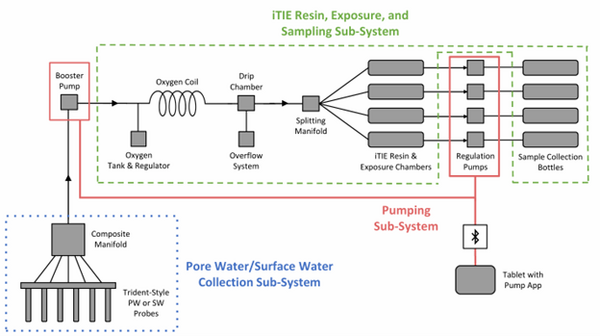
Figure 1: A schematic diagram of the iTIE system prototype. The system is divided into three sub-systems: 1) the Pore Water/Surface Water Collection Sub-System (blue); 2) the Pumping Sub-System (red); and 3) the iTIE Resin, Exposure, and Sampling Sub-System (green). Water first enters the system through the Pore Water/Surface Water Collection Sub-System. Porewater can be collected using Trident-style probes, or surface water can be collected using a simple weighted probe. The water is composited in a manifold before being pumped to the rest of the iTIE system by the booster pump. Once in the iTIE Resin, Exposure, and Sampling Sub-System, the water is gently oxygenated by the Oxygen Coil, separated from gas bubbles by the Drip Chamber, and diverted to separate iTIE Resin and Exposure Chambers (or iTIE units) by the Splitting Manifold. Water movement through each iTIE unit is controlled by a dedicated Regulation Pump. Finally, the water is gathered in Sample Collection bottles for analysis.
The latest iTIE prototype consists of an array of sorptive resins that differentially fractionate sampled water, and a series of corresponding flow-through organism chambers that receive the treated water in situ. Resin treatments can be selected depending on the chemicals suspected to be present at each site to selectively sequester certain chemical of concern (CoC) classes from the whole water, leaving a smaller subset of chemicals in the resulting water fraction for chemical and toxicological characterization. Test organism species and life stages can also be chosen depending on factors including site characteristics and study goals. In the full iTIE protocol, site water is continuously sampled either from the sediment pore spaces or the water column at a site, gently oxygenated, diverted to different iTIE units for fractionation and organism exposure, and collected in sample bottles for off-site chemical analysis (Figure 1). All iTIE system components are housed within waterproof Pelican cases, which allow for ease of transport and temperature control.
Porewater and Surface Water Collection Sub-system
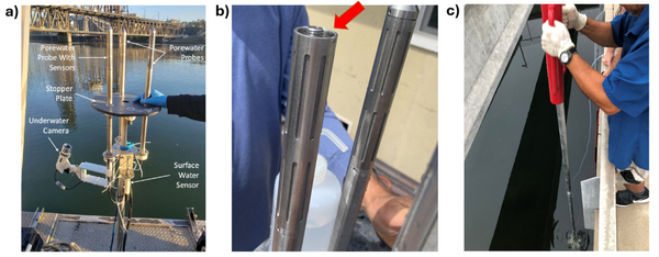
Figure 2: a) Trident probe with auxiliary sensors attached, b) a Trident probe with end caps removed (the red arrow identifies the intermediate space where glass beads are packed to filter suspended solids), c) a Trident probe being installed using a series of push poles and a fence post driver
Given the importance of sediment porewater to ecosystem structure and function, investigators may employ the iTIE system to evaluate the toxic effects associated with the impacted sediment porewater. To accomplish this, the iTIE system utilizes the Trident probe, originally developed for Department of Defense site characterization studies[8]. The main body of the Trident is comprised of a stainless-steel frame with six hollow probes (Figure 2). Each probe contains a layer of inert glass beads, which filters suspended solids from the sampled water. The water is drawn through each probe into a composite manifold and transported to the rest of the iTIE system using a high-precision peristaltic pump.
The Trident also includes an adjustable stopper plate, which forms a seal against the sediment and prevents the inadvertent dilution of porewater samples with surface water. (Figure 2). Preliminary laboratory results indicate that the Trident is extremely effective in collecting porewater samples with minimal surface water infiltration in sediments ranging from coarse sand to fine clay. Underwater cameras, sensors, passive samplers, and other auxiliary equipment can be attached to the Trident probe frame to provide supplemental data.
Alternatively, practitioners may employ the iTIE system to evaluate site surface water. To sample surface water, weighted intake tubes can collect surface water from the water column using a peristaltic pump.
Oxygen Coil, Overflow Bag and Drip Chamber
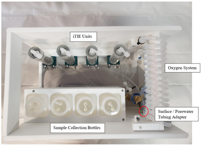
Figure 3. Contents of the iTIE system cooler. The pictured HDPE rack (47.6 cm length x 29.7 cm width x 33.7 cm height) is removable from the iTIE cooler. Water enters the system at the red circle, flows through the oxygen coil, and then travels to each of the individual iTIE units where diagnostic resins and organisms are located. The water then briefly leaves the cooler to travel through peristaltic regulation pumps before being gathered in sample collection bottles.
Porewater is naturally anoxic due to limited mixing with aerated surface water and high oxygen demand of sediments, which may cause organism mortality and interfere with iTIE results. To preclude this, sampled porewater is exposed to an oxygen coil. This consists of an interior silicone tube connected to a pressurized oxygen canister, threaded through an exterior reinforced PVC tube through which water is slowly pumped (Figure 3). Pump rates are optimized to ensure adequate aeration of the water. In addition to elevating DO levels, the oxygen coil facilitates the oxidation of dissolved sulfides, which naturally occur in some marine sediments and may otherwise cause toxicity to organisms if left in its reduced form.
Gas bubbles may form in the oxygen coil over the course of a deployment. These can be disruptive, decreasing water sample volumes and posing a danger to sensitive organisms like daphnids. To account for this, the water travels to a drip chamber after exiting the oxygen coil, which allows gas bubbles to be separated and diverted to an overflow system. The sample water then flows to a manifold which divides the flow into different paths to each of the treatment units for fractionation and organism exposure.
iTIE Units: Fractionation and Organism Exposure Chambers
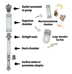
Figure 4. A diagram of the iTIE prototype. Water flows upward into each resin chamber through the unit bottom. After being chemically fractionated in the resin chamber, water travels into the organism chamber, where test organisms have been placed. Water is drawn through the units by high-precision peristaltic pumps.
At the core of the iTIE system are separate dual-chamber iTIE units, each with a resin fractionation chamber and an organism exposure chamber (Figure 4). Developed by Burton et al.[1], the iTIE prototype is constructed from acrylic, with rubber O-rings to connect each piece. Each iTIE unit can contain a different diagnostic resin matrix, customizable to remove specific chemical classes from the water. Sampled water flows into each unit through the bottom and is differentially fractionated by the resin matrix as it travels upward. Then it reaches the organism chamber, where test organisms are placed for exposure. The organism chamber inlet and outlet are covered by mesh to prevent the escape of the test organisms. This continuous flow-through design allows practitioners to capture the temporal heterogeneity of ambient water conditions over the duration of an in situ exposure. Currently, the iTIE system can support four independent iTIE treatment units.
After being exposed to test organisms, water is collected in sample bottles. The bottles can be pre-loaded with preservation reagents to allow for later chemical analysis. Sample bottles can be composed of polyethylene, glass or other materials depending on the CoC.
Pumping Sub-system
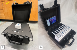
Figure 5. The iTIE system pumping sub-system. The sub-system consists of: A) a single booster pump, which is directly connected to the water sampling device and feeds water to the rest of the iTIE system, and B) a set of four regulation pumps, which each connect to the outflow of an individual iTIE unit. Each pump set is housed in a waterproof case with self-contained rechargeable battery power. A tablet is mounted inside the lid of the four pump case, which can be used to program and operate all of the pumps when connected to the internet.
Water movement through the system is driven by a series of high-precision, programmable peristaltic pumps (EcoTech Marine). Each pump set is housed in a Pelican storm travel case. Power is supplied to each pump by internal rechargeable lithium-iron phosphate batteries (Bioenno Power).
First, water is supplied to the system by a booster pump (Figure 5A). This pump is situated between the water sampling sub-system and the oxygen coil. The booster pump: 1) facilitates pore water collection, especially from sediments with high fine particle fractions; 2) helps water overcome vertical lifts to travel to the iTIE system; and 3) prevents vacuums from forming in the iTIE system interior, which can accelerate the formation of disruptive gas bubbles in the oxygen coil. The booster pump should be programmed to supply an excess of water to prevent vacuum formation.
Second, a set of four regulation pumps ensure precise flow rates through each independent iTIE unit (Figure 5B). Each regulation pump pulls water from the top of an iTIE unit and then dispenses that water into a sample bottle for further analysis.
Study Design Considerations
Diagnostic Resin Treatments
Several commercially available resins have been verified for use in the iTIE system. Investigators can select resins based on stressor classes of interest at each site. Each resin selectively removes a CoC class from site water prior to organism exposure.
Resins must be adequately conditioned prior to use. Otherwise, they may inadequately adsorb toxicants or cause stress to organisms. New resins should be tested for efficacy and toxicity before being used in an iTIE system.
Test Organism Species and Life Stages
Practitioners can also select different organism species and life stages for use in the iTIE system, depending on site characteristics and study goals. The iTIE system can accommodate various small test organisms, including embryo-stage fish and most macroinvertebrates. The following common toxicity tests can be adapted for application within iTIE systems[12].
Freshwater acute toxicity:
Freshwater chronic toxicity:
- Americamysis survival, growth and fecundity
- Atherinops affinis embryo-larval survival and growth
Acute toxicity is quantifiable via organism survival rates immediately following the termination of an iTIE system field deployment. Chronic toxicity can be quantified by continuing to culture and observe test organisms in-lab. Common chronic endpoints include stunted growth, altered development such as teratogenicity in larval fish, decreased reproduction rates, and changes in gene expression.
Several gene expression endpoints have been detectable in bioassays following an iTIE system deployment and in-lab culturing period. Steigmeyer et al.[2] were able to detect changes in the expression of two genes in D. magna after a 24-hour exposure to bisphenol A. In a separate study, Nichols[13] found a significant decline in acetylcholinesterase activity in H. azteca after a 24-hour exposure to chlorpyrifos. These results indicate a potential to adapt other gene expression bioassays for use in conjunction with iTIE system field exposures to prove stressor-causality linkages.
Cost Effectiveness Study
Burton et al.[1] conducted a cost effectiveness study comparing the iTIE technology with the traditional US EPA Phase 1 TIE method. Comparisons were based on the estimated time required to complete various sub-tasks within each method. Sub-tasks included organism care, equipment preparation, mobilization and deployment, test maintenance, test termination, demobilization, and test termination analyses. It was ultimately estimated that the iTIE protocol requires 47% less time (67 fewer hours) to complete than the Phase 1 TIE method, with the largest time differences in equipment preparation, deployment, test maintenance, and demobilization. It is important to note that the iTIE method may require additional initial costs for equipment and training.
Field Application
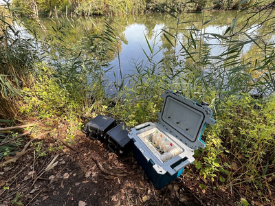
Figure 6. iTIES deployment at the Rouge River, Detroit, MI. In the foreground is the iTIE Cooler Sub-System, which contains iTIE resin treatments and test organism groups, as well as the oxygenation coil and sample collection bottles. Next to the iTIE Cooler are the two pump cases. The Trident can be seen above the pump cases, installed in the river channel near shore.
The iTIE system has been successfully deployed at a variety of marine and freshwater sites during the proof-of-concept phase of prototype development. One example is the 2024 iTIE system deployment completed near the mouth of the Rouge River in Detroit, MI (Figure 6). The Rouge River watershed has a long history of industrialization, with a legacy of chemical dumping, channelization, damming, and urban runoff[14]. This has led to degraded environmental conditions, with previous detections of a wide range of chemicals including heavy metals and various organics.
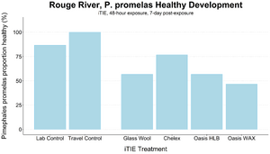
Figure 7. Survival and healthy development of
P. promelas embryos and larvae following a 48-hour iTIE exposure near the mouth of the Rouge River. Organisms were exposed to site porewater as embryos for 48 hours and cultured post-exposure for an additional 5 days.
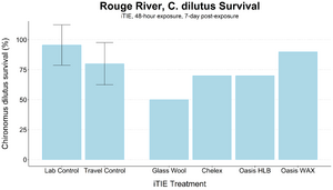
Figure 8. Survival of
C. dilutus larvae after an iTIE exposure near the mouth of the Rouge River. Organisms were exposed to site porewater for 48 hours and cultured post-exposure for an additional 5 days. Error bars show standard deviation.
An iTIE system deployment was designed and completed to determine which chemical classes are most responsible for causing toxicity at the site. Resin treatments included glass wool (inert, non-fractionating substance), Chelex (metals sorption), Oasis HLB (general organics sorption), and Oasis WAX (organics sorption, with a high affinity for PFAS). The study utilized fathead minnow (P. promelas) embryos, due to their relative sensitivity to metals and PAHs, as well as second-instar midge (Chironomus dilutus) larvae due to their relative sensitivity to PFAS.
The test organisms were exposed to fractionated porewater in situ for 48 hours. Following exposure, organisms were cultured for an additional five days, and survival was recorded (Figures 7 and 8). Moderate declines in survival were seen in both species in the glass wool treatment, indicating toxicity at the site. For P. promelas, the highest proportion of healthy development occurred in the Chelex treatment, supporting the hypothesis that metals are a dominant cause of toxicity. C. dilutus had the greatest survival in the Oasis WAX treatment, suggesting that an organic stressor class like PFAS is also present at harmful concentrations in the river.
Water chemical analyses of fractionated and unfractionated water samples were completed to support biological results. Analyses were conducted for a range of stressor classes including metals, PAHs, PCBs, an organophosphate pesticide (chlorpyrifos), a PFAS compound (PFOS) and a pyrethroid insecticide (permethrin). Of these analytes, only heavy metals and PFOS were detected. Some chemical classes including PAHs and PCBs were not detected at the site.
To reach similar conclusions using traditional Phase 1 TIE methods, one would need to complete the following tests: baseline toxicity, filtration, aeration, EDTA, C18 SPE, and methanol elution of C18 SPE. The iTIE method allows the same conclusions to be drawn with significantly less time and effort required.
Summary
The in situ Toxicity Identification Evaluation technology and protocol is a powerful tool that investigators can use to strengthen causal linkages between chemical stressors and ecological toxicity. By fractionating sampled water and exposing test organisms in situ, investigators can gather toxicity response data while minimizing sample manipulation and accurately representing environmental conditions.
References
- ^ 1.0 1.1 1.2 1.3 1.4 1.5 Burton, G.A., Cervi, E.C., Meyer, K., Steigmeyer, A., Verhamme, E., Daley, J., Hudson, M., Colvin, M., Rosen, G., 2020. A novel In Situ Toxicity Identification Evaluation (iTIE) System for Determining which Chemicals Drive Impairments at Contaminated Sites. Environmental Toxicology and Chemistry, 39(9), pp. 1746-1754. doi: 10.1002/etc.4799
- ^ 2.0 2.1 2.2 2.3 Steigmeyer, A.J., Zhang, J., Daley, J.M., Zhang, X., Burton, G.A. Jr., 2017. An in situ toxicity identification and evaluation water analysis system: Laboratory validation. Environmental Toxicology and Chemistry, 36(6), pp. 1636-1643. doi: 10.1002/etc.3696
- ^ United States Environmental Protection Agency, 2007. Sediment Toxicity Identification Evaluation (TIE) Phases I, II, and III Guidance Document, EPA/600/R-07/080. 145 pages. Free Download Report.pdf
- ^ In Situ Toxicity Identification Evaluation (iTIE) Technology for Assessing Contaminated Sediments, Remediation Success, Recontamination and Source Identification Project Website Final Report.pdf
- ^ Norberg-King, T., Mount, D.I., Amato, J.R., Jensen, D.A., Thompson, J.A., 1992. Toxicity identification evaluation: Characterization of chronically toxic effluents: Phase I. Publication No. EPA/600/6-91/005F. U.S. Environmental Protection Agency, Office of Research and Development. Free Download from US EPA Report.pdf
- ^ Burton, G.A. Jr., Nordstrom, J.F., 2004. An in situ toxicity identification evaluation method part I: Laboratory validation. Environmental Toxicology and Chemistry, 23(12), pp. 2844-2850. doi: 10.1897/03-409.1
- ^ Burton, G.A. Jr., Nordstrom, J.F., 2004. An in situ toxicity identification evaluation method part II: Field validation. Environmental Toxicology and Chemistry, 23(12), pp. 2851-2855. doi: 10.1897/03-468.1
- ^ Chadwick, D.B., Harre, B., Smith, C.F., Groves, J.G., Paulsen, R.J., 2003. Coastal Contaminant Migration Monitoring: The Trident Probe and UltraSeep System. Hardware Description, Protocols, and Procedures. Technical Report 1902. Space and Naval Warfare Systems Center.
- ^ Woodard, S., Mohr, T., Nickelsen, M.G., 2014. Synthetic media: A promising new treatment technology for 1,4-dioxane. Remediation Journal, 24(4), pp. 27-40. doi: 10.1002/rem.21402
- ^ Lemos, B.R.S., Teixeira, I.F., de Mesquita, J.P., Ribeiro, R.R., Donnici, C.L., Lago, R.M., 2012. Use of modified activated carbon for the oxidation of aqueous sulfide. Carbon, 50(3), pp. 1386-1393. doi: 10.1016/j.carbon.2011.11.011
- ^ Iannone, A., Carriera, F., Di Fiore, C., Avino, P., 2024. Poly- and Perfluoroalkyl Substance (PFAS) Analysis in Environmental Matrices: An Overview of the Extraction and Chromatographic Detection Methods. Analytica, 5(2), pp. 187-202. doi: 10.3390/analytica5020012 Open Access Article
- ^ U.S. Environmental Protection Agency, Office of Solid Waste and Emergency Response, 1994. Catalogue of Standard Toxicity Tests for Ecological Risk Assessment. ECO Update, 2(2), 4 pages. Publication No. 9345.0.05I Free Download Report.pdf
- ^ Nichols, E., 2023. Methods for Identification and Prioritization of Stressors at Impaired Sites. Masters thesis, University of Michigan. University of Michigan Library Deep Blue Documents. Free Download Report.pdf
- ^ Ridgway, J., Cave, K., DeMaria, A., O’Meara, J., Hartig, J. H., 2018. The Rouge River Area of Concern—A multi-year, multi-level successful approach to restoration of Impaired Beneficial Uses. Aquatic Ecosystem Health and Management, 21(4), pp. 398-408. doi: 10.1080/14634988.2018.1528816
See Also


